Experimental Comparison of Five Approximation Algorithms for

International Journal of u- and e- Service, Science and Technology Vol. 7, No. 6 (2014), pp. 69-84 http://dx.doi.org/10.14257/ijunesst.2014.7.6.07

Experimental Comparison of Five Approximation Algorithms for Minimum Vertex Cover Imran Khan and Sangeen Khan Department of Computer and Software Technology, University of Swat, KPK, Pakistan, [email protected], [email protected] Abstract Numerous approximation algorithms have been presented by researchers for approximation of minimum vertex cover, all of these approaches have deficiencies in one way or another. As minimum vertex cover is NP-Complete so we can’t find out optimal solution so approximation is the way left but it is very hard for someone to decide which one procedure to use, in this comparison paper we have selected five approximation algorithms and have drawn detailed experimental comparison. Best available benchmarks were used for the comparison process which was to compare multiple algorithms for the same task on different aspects. Extensive results have been provided to clarify the selection process, probability of production optimal solutions, run time complexity and approximation ratio were factors involved in the process of selection. Keywords: Keywords: MVC (Minimum vertex cover), MIS (Maximum independent sets), DCA (Degree Contribution Algorithm), VSA (Vertex Support Algorithm), DC (Degree Contribution), MWVC (Minimal Weighted Vertex Cover), And MWIS (Maximal Weighted Independent Set)

1. Introduction Approximation algorithms play a critical role in obtaining near to optimal solution to all NP-Complete problems, these problems are intractable and we can‟t find out optimal solution in polynomial time. This strong belief of computer science community about NPCompleteness compelled researchers to come out with new techniques, of them approximation is one of the best approach. Another approach is heuristics but it has no guarantee of producing quality solution in reasonable time. Most of NP-Complete problems are modeled in graphs and minimum vertex cover is one of the problems where objective is to find out the minimum number of vertices to cover the whole graph. Graph G (V, E) is combination of nodes and edges where nodes are connected through edges. After modeling the input problem over graph, it is then manipulated in several ways depends on the final objective. Application areas of graph theory includes bioinformatics, biochemistry, logistic networks, social science, electrical engineering, digital electronics etc. [1] All algorithms that adopts approximation approach can be efficiently judged on the basis of ratio between their solution and optimal actual solution, the minimum it is the good the algorithm is. Mathematically ρ i = A (i)/OPT (i) ≥ 1. When ρ i =1 then the approximate solution is actual optimal solution, but this is not the case always because these problems are intractable and according to Gray & Johnson a problem as intractable if it is so hard that no polynomial algorithm can possibly solve it [2]. The value of ρi determines the quality of solution, the more it diverts from 1 the more solution degrades. Basically there are two

ISSN: 2005-4246 IJUNESST Copyright ⓒ 2014 SERSC

International Journal of u- and e- Service, Science and Technology Vol. 7, No. 6 (2014)

different versions of graph related problems one is decision version and other one is optimization. In decision version a try is made to answer a question, like is there exist such a solution that the whole graph is covered with „k‟ nodes etc. In this version just a check is made to answer this, while in optimization version a search is made for the optimal solution as much possible. Here we will deal with optimization version to find out the most optimal solution possible for a problem. Vertex cover is one of the graph related problem where the objective is to extract a set of vertices in a specific graph which cover all the edges of the graph. Minimal vertex cover is just the same but here another objective is to optimize the solution such that the total vertices in the vertex cover set remains as minimum as possible, Let a Graph G (V, E) where ‘ V’ represent vertices and ‘ E’ represent edges then minimal vertex cover vertices are such that Vc⊆ V which cover all the edges in the graph. In 1972, Richard Karp showed that finding the solution of minimal vertex cover in a graph is an NP-complete problem [3]. Vertex cover remains NP-complete even in cubic graphs [4] and even in planar graphs of degree at most 3 [5]. Li et al. argued that current heuristic algorithms of MVC only consider vertex features in isolation in order to decide whether a vertex is in or not in the solution set [6]. Independent set problem also belongs to NP complete and these both problems can be easily solved with just one solution [Reference]. Independent set is a set of nodes which share no each with each other and in maximum independent set search is made to maximize total number of independent nodes as much as possible. Practically the nodes other than MVC are MIS nodes and vice versa. Maximum clique is also one of the related NP-Complete problem where the objective is to find out maximum number of nodes which are completely connected to each other, in simple words this is complement of maximum independent set and the rule hold opposite direction too. Comparison parameters that we have selected here are runtime complexity, approximation ratio and the probability of producing optimal solution which leads to accurate operational decision in any field. Run time complexity is the total number of basis operations involved in solving a problem but here we will only encounter worst case complexity as this shows a peak value of an algorithm to be worst. Approximation ratio as mentioned above shows how much the solution is diverted from the original one, the greater it is the worst the solution is. The actual probability of an algorithm to find out optimal solution can be guessed by obtaining the percentage of approximation solution equal to optimal solution in a set of well-defined benchmarks, and for this we have collected best heterogeneous benchmarks available across the repository of internet. This comparison will help businesses and all other fields where MVC, MIS and clique application exist as these three problems are easily reducible to one another and vice versa.

2. Literature Review R Karp proved that Minimal vertex cover is NP-Complete [3]. This means that we cannot find an optimal solution in polynomial time for the minimal vertex cover problem until it is proved that P=NP. Vertex cover problem has received considerable attention from researchers and scientists in the last decade due to its potential for enormous and wide-range of applications. Chavatal proposed a simplest approximation algorithm for MVC named “Maximum degree Greedy” which a vertex randomly to be in MVC set, all adjacent edges are deleted and the process continues till no edge remains [7]. This was not a good approach because selection of node for MVC needs quite intelligent guess not a random guess. Clarkson modified this random approach and random selection was changed with selection made on the basis of degree [8]. Halldorsson and Radhakrishnan took a greedy approach

70

Copyright ⓒ 2014 SERSC


when they proposed an algorithm for Maximum independent set (MIS) called Greedy Independent Cover (GIC) [11]. They added minimum degree node to MIS. MIS is also NPComplete problem [1] and there is a simple reduction from MIS to MVC. i. e. all the vertices that are not in independent set are in MVC. This approach identifies an important property of graphs for calculation of minimum vertex cover. The chances for selection of a node in optimal vertex cover that has minimum degree are very low. The same fact was exploited with some added optimization by several other researchers. They proved that GIC can find optimal solution for trees and therefore in paths. Delbot and Laforest have shown that on average, GIC performs better than other algorithms in terms of quality, but its performance is worst for the average worst case graphs [9]. They have also noted after various experimentation of GIC on several categories of graphs that error percentage never exceeds more than 25 [9]. In comparison to other techniques, GIC can be reliably used on general graphs but then we have to compromise with the worst case complexity returned on average worst case graphs which is not a norm in practice. These algorithms (MDG and GIC) are the simplest algorithms in every respect like design, decision process and running time. Avis and Imamura devised a List left heuristic approach for solving MVC with maximum approximation ratio of √ Δ /2+3/2 and minimum ratio of√ (∆/2) where „∆‟ is the maximum degree in the graph [12]. They also prove that √ Δ /2 is the least approximation ratio for any sort list algorithm that is applied to find solution of minimum vertex cover problem. They make use of list heuristics and makes decision on the information available for a particular instance. All nodes are first sorted in decreasing order by their degrees and for each node, the decision of including or excluding this node to the MVC is made on the basis of incident edges. If a node has incident edge and is not yet covered then that node is selected for minimal vertex cover. But when this method was applied and analyzed in experimental settings considering various type of graphs [9], it became obvious that this list heuristic cannot provide better or even comparable solution to the other greedy approaches in general. An Annealing algorithm for finding out minimum vertex cover was proposed by Xu and Ma [16] they have proposed the adoption of a new acceptance factor for deciding about the solution for minimum vertex cover problem. They call each vertex a neuron and total number of neurons are equal to the total number of vertices in a graph. The layout of their algorithm is like an iterative improvement algorithm and the only change is that the cost increasing transitions are also accepted with cost decreasing transitions. Starting with an initial solution, a neighbor solution is generated. If reduction in the cost is found then existing solution is replaced by the newly produced solution. But if no reduction in cost is found then the decision of keeping or discarding this new solution is made on the basis of specific probability. The effectiveness of algorithm is demonstrated by providing implementation results with some benchmarks. Although their approximation ratio is near 100% for few benchmarks but the number of applied benchmarks are not extensive so it is difficult to judge their performance for different graph types. Plus they have also not provided any pseudo code that could have been helpful for other researchers to implement and test the approach for the comparison purpose. Delbot and La forest presented another list heuristic for vertex cover named List Right [13]. This approach is based on technically similar List Left that was presented by Avis and Imamura [12]. By introducing slight modifications in the original paper, they have been able to receive better result ratio. This approach gives an approximation ratio of „∆‟ at worst case, where „Δ‟ is the maximum degree in the graph. List right works by scanning the list of vertices from right to left and making decisions for the currently scanned vertex for selection for MVC. If the currently scanned vertex has at least one right neighbor that is not in vertex cover then the currently scanned vertex is selected for vertex cover. The problem of scanning


71


vertices from one direction to another is same as List Left. The technique applied in List right can be extended to the scenarios where graphs are processed online and nodes are added and deleted on the fly. Experimental results of list right carried out by Delbot and Laforest have shown that list right outperforms list left on all graphs and the maximum percentage error of list right never exceeds than that of 55% and even in worst case graphs, list right provides better results among other techniques analyzed [9]. The main feature of this approach is that it takes decision on the basis of already scanned vertices. Aggression and Stein presented a divide and conquer approach but their approach does not seem to be feasible for practical purpose as the criteria for graph division is vague 17]. The idea is to divide the graph into sub graphs and then solving each sub graph. The sub-solutions are then combined to get the solution of the original graph. The division of graph is done on the basis of specific graph structure and unique properties. This specific division is done for the sake of trimming computation effort. The included methodologies are degree one and two vertices elimination, triangle elimination, almost bipartite etc. Their algorithm offers no specific approximation ratio. In fact it depends on the methodology applied for the division of graph into sub graphs. Divide and conquer approach is very efficient for providing solutions to other scenarios it fails to provide a generic solution plus the graph divisions also add to the complexity. Balaji et al. devised a new approach with new data structure named support of a vertex [14]. All decisions regarding vertices are made on the basis of this value. Support of vertex that they proposed is the sum of degrees of all vertices adjacent to a vertex. They have tested their approach on large number of benchmarks and are optimal in most of the cases and its rum time complexity is O (EV2). VSA is optimized by Imran and Hasham by modifying the decision of MVC node selection and named it MVSA, the initial selection was on the basis of maximum vertex support while MVSA select node on the basis of their surroundings [18]. A new clever intelligent greedy approach is presented by Gajurel and Bielefeld named NOVAC-1[15]. This approach works on a clever concept raised from the keen observation and analysis of relationship among vertices. The vertices attached to minimum degree nodes are candidate of MVC with high probability. A well modified version of VSA named AVSA has been proposed by [19] and has shown that their modification has made the stated previous approach efficient.

3. The Algorithms This section includes description of algorithms which have been selected for the comparison process against minimum vertex cover. 3.1. Maximum Degree Greedy (MDG) Chavatal proposed a simple approximation algorithm that was based on the random approach i. e. the fate of vertex for possible inclusion in MVC was based on the minimal available information [7]. The algorithm selects a single vertex through random approach in the input graph for every iteration. Then this random node is added to the MVC and all its adjacent edges are deleted. The process is terminated when no edge remains in the graph. Later it was modified by Clarkson [8], he noticed that those nodes of a graph have high probability of inclusion in the vertex cover that have the maximum degree among all vertices. So, he opted for a stepping approach where at each step he would select the node with the maximum degree and then would drop the entire edges incident on that vertex. The process continues till no edge remains. This algorithm is known as Maximum Degree Greedy (MDG) and the complexity of this algorithm is O (E2) where E is the total number of Edges in the graph. Experimental analysis carried out by Delbot and Laforest have shown that MDG gives

72



a max of 33% error on ErdosRenyi graphs, 9% on trees, 44% on Bhoslib, 32% on regular graphs and 70% on average worst case graphs. Worst case graphs are those that are designed to trap an algorithm [9]. Error percentage is high because every time the vertex with maximum degree is not the one to be in Minimal vertex cover set, it will affect all the other future MVC nodes. As the algorithm we proposed in this article is based on greedy approach, we will first present literature related to the greedy approaches. The below is pseudo code of the simple MDG approach as discussed above. Maximum-Degree-Greedy (Graph G) { C ←∅; //initially no vertex is in vertex cover set While E! =∅ do Select a vertex u of maximum degree; V ← V − {u}; C←C ∪ {u}; Drop all edges of u End; Return C; }; The degree for each vertex is calculated in each step to identify a vertex with maximum degree for the next step. As degrees are calculated using network bench model (Degree Calculation Model) so it calculates it in a total of O (E) steps. The main loop also executes „E‟ times and the operations take a constant basis operation and thus have a constant run time. The total run time complexity for Maximum degree greedy is O (E2) in worst case. This approach fails on various graphs in producing optimal solution presented in the literature. 3.2. Vertex Support Algorithm (VSA) A different approach is proposed by Balaji, Swaminathan and Kannan [14] that selects vertices for MVC on the basis of new criteria named support of a vertex. They define support of vertex as sum of degrees of all adjacent vertices to a vertex. Here they have used a new technique for the selection criteria of vertex for inclusion into MVC. In this approach, support of a vertex is actually the sum of degrees of vertices adjacent to that vertex. i.e Support (V) =S (V) =∑ _(u ∈N)G(v)d(u). The vertex which has maximum support value is selected for MVC and all edges incident on that node are deleted. The same process is repeated till all edges are processed in the graph. They have shown the effectiveness of algorithm by providing empirical results obtained using extensive set benchmark graphs. They have also compared their approach with other techniques. The algorithm design is a bit complex and the calculation of support for each and every node in iterative manner adds to the complexity but the quality of results is considerably better than other approaches. Run time complexity of this algorithm is O (E.V2), where „E‟ is total number of Edges and „V‟ is total number of vertices in the graph. VSA also based on greedy methodology. The pseudo code for VSA is as under.

Vertex-Support-Algorithm (Graph g) { Repeat while E ≠ ϕ Step 1: Calculate Degree of each vertex.


73


Step 2: Calculate Support of each vertex which is sum of degrees of adjacent vertices to that vertex. Step 3: Add the vertex with maximum value of Support to „Vertex Cover‟ and if more than one vertex have same max value then add one which has higher degree. Step 4: Delete all adjacent edges to that vertex by putting 0‟s in adjacency matrix. End; Return „Vertex Cover‟; }; Its only flaw is probably the run time complexity. This method is more suited for finding MVC for small or medium sized graphs. 3.3. Nearly Optimal Vertex Cover (NOVAC-1) Gajurel and Bielfeld presented a clever and simple technique named as NOVAC-I that is based on very important concept of analyzing the relationship among vertices [15]. While analyzing the relationship between a vertex and its probability to be a part of MVC, they observed that those vertices are high probable candidates for MVC that are connected to the minimum degree vertex. The algorithm they have developed works by selecting those vertices in vertex cover that are adjacent to minimum degree vertex. First, degree of each vertex is calculated and then sum of degree of adjacent vertices is also calculated for each vertex. Vertices are processed in increasing order by their degrees. Vertex with minimum degree is selected for further processing and all its adjacent vertices are added to minimum vertex cover. If there are more than one vertex that have the same minimum degree value then selection is based on the value of the sum of the adjacent vertices degrees. A vertex that has maximum adjacent value is selected and all adjacent vertices are added to vertex cover. The process repeats till no edge remains. At the end minimum vertex cover is obtained. The analysis of this approach in experimental settings carried out in [14] provided the information that this approach only provides an average of 35% optimal results. But a positive note is that the approximation ratio never exceeds 1.077 and the average approximation ratio is 1.008. This is also a greedy approach but there are some modifications to handle the changes in graph. NOVAC-I-Algorithm (Graph g) { Initialize VC to „0‟; //VC means vertex cover set. Step 1: Calculate degree for each vertex in the graph. Step 2: Calculate the sum of degrees of adjacent vertices for each vertex. Repeat while all Edges are processed. { Step 3: Get a vertex with minimum degree, and if there are more than one vertex with minimum degree the select the one having maximum value of sum of degrees of adjacent vertices. Step 4: Add all adjacent vertices of that vertex to vertex cover and delete all its edges. Step 5: Update value of degrees and sum of degrees of adjacent vertices for each vertex. } }; Run time complexity using their approach is in O (n2log n) where „n‟ is total number of vertices. 3.4. Advanced Vertex Support Algorithm (AVSA)

74



A modified version of VSA have been proposed in [19] and have showed that if the selection is modified then results vary a lot from the original values. Conclusion drawn from this is that not only the data structure affects the final values but the way how we manipulate that is also most important one. AVSA (Graph G) { MVC [], D [], S [], min_support [], While (Edges ≠ ∅) { For each v V calculate degree of v // calculate degree for each node in the graph. For each v V Calculate support value for each v that isS (V) = . Find out all nodes with minimum support value and add it to „min_support‟ Find out neighbors to all nodes in „min_support‟. Find node with maximum support value in neighbors of „min_support‟. Add it to MVC, Drop all its edges. } } 3.5. Modified Vertex Support Algorithm (MVSA) MVSA (Modified vertex support algorithm) is a modified form of VSA that was proposed by Imran and Hasham [18] in which they have modified the way vertices are chosen for minimum vertex cover. The original method was solely dependent on greedy methodology in which they selected vertex on the basis of maximum support. The change was made in the selection process and rather than selecting vertex just on the basis of maximum support, MVSA selects vertex after analysis of surrounding support value of all attached vertices to the candidate node. All vertices attached to minimum support value is analyzed first on the basis of their support value and then vertex with maximum support is selected. This change although seems to be a small modification but experimental results provided in [14] show that MVSA can provide better results in comparison to the original VSA proposed. The pseudo code of MVSA is as under: MVSA (Graph G) { MVC [], D [], S [], min_support [] While (Edges ≠ ∅) { For each v ∈ V calculate degree of v // calculate degree for each node in the graph. For each v ∈ V Calculate support value for each v that is S (V) =∑ (u∈N)〖 (v〗 )d(u). Find out all nodes with minimum support value and add it to „min_support‟


75


Find out neighbors to all nodes in „min_support‟. Find node with minimum support value in neighbors of „min_support‟. Add it to MVC, Drop all its edges. } } There is no extra complexity involved in computation and decisions are quite straight forward. Run time complexity of the proposed algorithm is in O (EV log v).

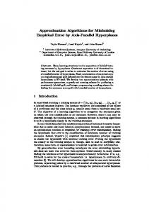
4. Experimental Comparison For the sack of comparative analysis we have encountered approximation ratio, percent of producing optimal solution against benchmarks and run time complexity. Approximation ratio is actually the ratio of diversion from the optimal value, if it is equal to 1 means the produced solution is optimal, the more it deviates from 1 shows that solution is diverting from the original value. In addition to this the capability of an algorithm to produce optimal solution in overall benchmarks tested is measured and represented in terms of percentage. Run time complexity is the total number of basic operations that is used by a technique to solve an input problem. In analysis of algorithms we usually take care of worst case complexity because it can be total number of maximum operations that an algorithm can perform. 4.1. Capability of Producing Optimal Solutions The criteria for calculating percentage is a little bit stupid but if analyzed in the set of well collected benchmarks can produce optimal percentage ratio nearly equal to the real world scenario. For the sake of this perfection all benchmarks used in this article for comparative analysis we tried to collect all best benchmarks. The total number of solution equal to optimal solution in terms of percent to total benchmarks is calculated from the table given below which contains results of algorithms used in comparative analysis against benchmarks with known optimal solution and total number of nodes in that graph. All algorithms selected for comparison are checked against the collection of benchmarks and the data was collect in the table 1 which shows all benchmarks, their total number of nodes, optimal solution and solution produced by each algorithm in the set. For clarification we converted the information of table1 in terms of optimal solution percentage and graph given in figure 1 shows these percentage values.

Figure 1. Optimal Solution Percentage

76



According to information given in figure1 VSA is able to produce optimal solution in almost 73.33% of benchmarks and is highest percentage among all. NOVAC-I, MVSA,AVSA produced optimal solution in approximately 53.33% of benchmarks tested while MDG lies in the last category by producing optimal solution with just 46.67% approximately. Here from total percentage one can decide which algorithm is better but just the total percentage is not important, we have other factors that‟s why we have done a full fletched combine comparison on these different factors. The probability of producing optimal solutions for VSA, AVSA, MVSA, NOVAC-I and MDG is 0.7, 0.5, 0.5, 0.5 and 0.4 respectively. According to the above calculation of probability VSA is capable of extracting optimal solution for MVC with a very high probability among others but as mentioned earlier this is just the single factor. The probability of producing wrong solution for VSA is 0.3 which is very less but approximation ratio there is of great importance, though it can product optimal solution with a very high ratio but if the approximation ratio is far greater the rest of solution then this carry no worth. The combined comparison is done in the last part of this article which tries to visualize all these factors. MDG is as one of the simplest algorithm but one of the worst too in producing solutions. Table 1. Benchmarks, their Total Nodes and known Optimal Solutions with Results of Algorithms Benchmarks

Total Vertices

Optimal MVC

MDG

VSA

NOVAC-1

AVSA

MVSA

graph50_6

50

38

38

44

38

38

38

graph50_10

50

35

35

41

35

35

35

graph100_1

100

60

60

95

60

60

60

graph100_10

100

70

70

96

70

70

70

graph200_5

200

150

150

184

150

150

150

graph500_1

500

350

350

485

350

350

350

graph500_2

500

400

400

484

400

400

400

graph500_5

500

290

290

454

290

290

290

phat300_1

300

292

293

292

293

294

294

phat300_2

300

275

278

275

275

279

279

phat300_3

300

264

269

264

266

272

272

phat700_1

700

689

693

692

692

692

692

phat700_2

700

656

660

656

657

660

660

phat700_3

700

638

642

639

641

649

649

jhonson8_2_4

28

24

24

24

24

24

24

jhonson8_4_4

70

56

62

56

56

56

56

jhonson16_2_4

120

112

112

112

112

112

112

jhonson32_2_4

496

480

480

480

480

480

480

sanr200-0.7

200

182

184

182

185

186

186

sanr200-0.9

200

158

164

158

159

163

163

sanr400_0.5

400

387

392

387

388

389

389

sanr400_0.7

400

379

384

397

381

381

381


77


fbr_30_15_5

450

420

429

429

424

424

424

fbr_35_17_2

595

560

570

573

565

565

565

c 125

125

91

93

91

92

92

95

c 250

250

206

211

206

211

211

211

c500.9

500

≤443

453

443

449

449

449

broc200_2

200

188

192

188

190

191

191

broc200_4

200

183

188

183

192

185

193

gen200_p0.9_44

200

156

165

156

163

160

166

Hamming6_2

64

32

32

32

32

32

32

Hamming6_4

64

60

60

60

60

60

60

Hamming8_2

256

128

128

128

128

128

128

Hamming8_4

256

240

248

240

240

240

240

Hamming10_2

1024

512

512

512

512

512

512

dsjc500

500

487

491

487

488

489

489

keller4

171

160

164

160

164

160

160

keller5

776

749

764

749

761

754

754

cfat200_1

200

188

188

188

188

188

188

cfat200_2

200

176

176

176

176

176

176

cfat200_5

200

142

142

142

142

142

142

cfat500_1

500

486

486

486

486

486

486

cfat500_2

500

474

474

474

474

474

474

cfat500_5

500

436

436

436

436

436

436

mann_a27

378

252

261

253

253

253

253

Figure 2. Probability of Producing Optimal Solutions 4.2. Comparison on the Basis of Approximation Ratio The ratio of calculated solution and actual optimal solution termed as approximation ratio, if it is equal to 1 then the produced solution is optimal. Mathematically „Pi= A (i)/Opt( i)‟, where „A(i)‟ represents approximate solution and „Opt(i)‟ represents

78



optimal solution. The value of „Pi‟ indicates the severity of diversion from the optimal solution, the more it is greater than „1‟ the worst the solution is. As we have collected all possible best benchmarks available so approximation ratio produced by the algorithms against these will almost near to practical scenarios. For the sack of clear representation of capability and behavior of an algorithm we have also calculated worst case approximation ratio and average case approximation ratio which shows how much an algorithm can give wrong solution approximately. Figure 3 shows the approximation ratio produced by these algorithms.

Figure 3. Approximation Ratio of Selected Algorithms against Benchmarks Straight line in Figure 3 shows the accuracy of an algorithm, the more it has variations the more different solution will be. Information reflected from Figure 3 shows that AVSA and MDG are more stable as compared to other three. Largest variation has been noted in VSA where at start of the line and then the solution is a little bit stable and reliable, the case is same with NOVAC-I where number of variations are smaller but their amplitude is far greater than any of these algorithms. Table 2 shows the approximation ratio produced by these algorithms as applied against the selected benchmarks. First column contains benchmark name, total nodes and approximation ratio produced. Analysis of data give in table 2 shows that worst case approximation ratio for AVSA, MDG, MVSA, NOVAC-1 and VSA are 1.032, 1.107, 1.064, 1.049 and 1.583 respectively. The worst one among these algorithms is VSA which give maximum approximation ratio while solving these benchmarks. This comparison is shown graphically with the help of graph given in Figure 4. Table 2. Algorithms and Benchmarks with their Approximation Ratios Approximation Ratio Benchmarks

Total Vertices AVSA

MDG

MVSA

NOVAC-1

50

1

1

1.000

0

1.158

graph50_10

50

1

1

1.000

1

1.171

graph100_1

100

1

1

1.000

1

1.583

graph100_10

100

1

1

1.000

1

1.371

graph200_5

200

1

1

1.000

1

1.227

graph500_1

500

1

1

1.000

1

1.386

graph50_6


VSA

79


80

graph500_2

500

1

1

1.000

1

1.210

graph500_5

500

1

1

1.000

1

1.566

phat300_1

300

1.007

1.003

1.003

1.000

phat300_2

300

1.015

1.011

1.015

1

1.000

phat300_3

300

1.03

1.019

1.030

1.008

1.000

phat700_1

700

1.004

1.006

1.004

1.004

1.000

phat700_2

700

1.006

1.006

1.006

1.002

1.000

phat700_3

700

1.017

1.006

1.017

1.005

1.000

jhonson8_2_4

28

1

1

1.000

1

1.000

jhonson8_4_4

70

1

1.107

1.000

1

1.000

jhonson16_2_4

120

1

1

1.000

1

1.000

jhonson32_2_4

496

1

1

1.000

1

1.000

sanr200-0.7

200

1.022

1.011

1.022

1.016

1.000

sanr200-0.9

200

1.032

1.038

1.032

1.006

1.000

sanr400_0.5

400

1.005

1.013

1.005

1.003

1.000

sanr400_0.7

400

1.005

1.013

1.005

1.005

1.047

fbr_30_15_5

450

1.01

1.021

1.010

1.01

1.021

fbr_35_17_2

595

1.009

1.018

1.009

1.009

1.023

c 125

125

1.011

1.022

1.044

1.011

1.000

c 250

250

1.024

1.024

1.024

1.024

1.000

c500.9

500

1.014

1.023

1.014

1.014

1.000

broc200_2

200

1.016

1.021

1.016

1.011

1.000

broc200_4

200

1.011

1.027

1.055

1.049

1.000

gen200_p0.9_44

200

1.026

1.058

1.064

1.045

1.000

Hamming6_2

64

1

1

1.000

1

1.000

Hamming6_4

64

1

1

1.000

1

1.000

Hamming8_2

256

1

1

1.000

1

1.000

Hamming8_4

256

1

1.033

1.000

1

1.000

Hamming10_2

1024

1

1

1.000

1

1.000

dsjc500

500

1.004

1.008

1.004

1.002

1.000

keller4

171

1

1.025

1.000

1.025

1.000

keller5

776

1.007

1.02

1.007

1.016

1.000

cfat200_1

200

1

1

1.000

1

1.000

cfat200_2

200

1

1

1.000

1

1.000

cfat200_5

200

1

1

1.000

1

1.000

cfat500_1

500

1

1

1.000

1

1.000

cfat500_2

500

1

1

1.000

1

1.000

cfat500_5

500

1

1

1.000

1

1.000

mann_a27

378

1.004

1.036

1.004

1.004

1.004



Figure 4. Worst Case Approximation Ratio Comparison The graph show in Figure 4 clearly visualize that AVSA is able to produce minimum worst case approximation ration in contrast to other approaches. VSA and AVSA are same algorithms, both make use of same data structures but the way that vertices are choose diverts the solutions towards optimal ones. Average case analysis of the approximation ratios given in Table 2 results that AVSA, MDG, MVSA, NOVAC-1 and VSA can produce average approximation ratios of 1.006, 1.013, 1.009, 1.006 and 1.061 respectively. On average AVSA and NOVAC-1 can perform best as compared to others. The average case comparison analysis is shown in figure 5. Graph give in figure 5 witness that AVSA is one of the best comparing other ones, the case is same with NOVAC-1. 4.2. Comparison on the Basis of Run Time Complexity The mathematical representation of total number of basis operations performed by an algorithm for solving an input problem instance is known as run time complexity. To provide independency from architectural issues theoretical scientists have assumed an ideal machine used for analysis of algorithms, that ideal machine is known as RAM (Random Access Machine) which have infinite memory and instructions are executed each by each in a sequential manner. This assumption made the analysis completely independent of operating system issues, hardware and other technical problems.

Figure 5. Average Case Approximation Ratio


81


Regarding the problem domain there are three types of run time complexities including best case, average case and worst case. Best case represent the total possible minimum number of operations performed by an algorithm to solve input problem instance, average case is average number of operations and worst case is the possible maximum number of operations. Table 3 presents algorithms with their worst case run time complexity. Table 3. Run Time Complexity of Selected Algorithms Algorithms Maximum degree greedy NOVCA-I VSA MVSA AVSA

Runtime Complexity n2 n2 log n n2 n2 n2

From run time complexity point of view NOVAC-I is worst algorithm among others, the rest of algorithms have same run time complexity means they perform same number of operations.

5. Conclusion Various algorithms have been analyzed by applying them to extensive benchmarks available across the internet. Efforts have been made to collect best of them which can give real idea about an algorithm. The analysis was based on percentage of producing optimal solutions, approximation ratio produced and their worst case running time complexity. According to the optimal solution percentage factor VSA is desirable algorithm capable of solving almost 73% of benchmarks optimally, this is a very big ratio as just 27% were left unsolvable in accordance to optimal one. Though VSA can produce optimal solution with high probability but it is also the fact that VSA is one of the worst algorithm according to analysis based on worst case approximation ratio. This means that either you will get optimal solution or the worst one but worst one can be in rare cases as compared to optimal ones. AVSA on the other hand managed to solve just 53% of benchmarks optimally but on both average and worst case analysis of approximation ratio support AVSA for producing best results. MDG, NOVAC-1 and MVSA were the flop one as they perform badly in fight against benchmarks for extracting minimum vertex cover. The final conclusion is to tradeoff between AVSA and VSA. If you need accuracy the VSA can give you optimal solution with high probability but is not reliable on the other hand AVSA is reliable one as either it will produce optimal solution or solution very near to optimal one so AVSA is desirable to be used in practical environment.

References [1] J. Chen, X. Huang, I. Kanj and G. Xia, “Linear FPT reductions and computational lower bound”, Proceedings of 36th ACM symposium on Theory of computing, (2004), Berlin Heidelberg. [2] M. Gary and D. Johnson, “Computers and intractability”, New York: Freeman, (1979). [3] R. Karp, “Reducibility among combinatorial problems”, New York: Plenum Press, (1972). [4] E. Demaine, “Sub exponential parameterized algorithms on bounded-genus graphs and H Minor-free graphs”, Journal of the ACM (JACM), vol. 52, no. 6, (2005), pp. 866-893. [5] I. Dinur and S. Safra, “On the hardness of approximating minimum vertex cover”, Annals of Mathematics, no. 162, (2005), pp. 439-485.

82



[6] S. Li, “An Approximation Algorithm for Minimum Vertex Cover on General Graphs”, in Proc. 3rd International Symposium: Electronic Commerce and Security Workshops (ISECS ’10), China: Academy, (2010), pp. 249-252. [7] V. Chvatal, “A Greedy Heuristic for the Set-Covering Problem”, Mathematics of Operations Research, vol. 4, (1979). [8] K. Clarkson, “A modification to the greedy algorithm for vertex cover problem”, Information Processing Letters, vol. 16, (1983). [9] F. Delbot and C. Laforest, “Analytical and experimental comparison of six algorithms for the vertex cover problem”, Journal of Experimental Algorithmics, vol. 15, (2010). [10] T. H. Cormen, C. E. Lieserson, R. L. Rivest and C. Stein, “Introduction to Algorithms”, 3rd Ed, MIT Press England, (2009). [11] M. Halldorsson and J. Radhakrishnan, “Greed is good: Approximating independent sets in sparse and bounded-degree graphs”, In Proceedings of 26th Annual ACM Symposium on Theory of Computing, (1994), New York: ACM. [12] D. Avis and T. Imamura, “A List Heuristic for Vertex Cover”, Operations research letters, vol. 35, (2007). [13] F. Delbot and C. Laforest, “A better list heuristic for vertex covers”, Information Processing Letters, vol. 107, (2008). [14] S. Balaji, V. Swaminathan and K. Kannan, “Optimization of Un-weighted Minimum Vertex Cover”, World Academy of Science, Engineering and technology, vol. 67, (2010). [15] S. Gajurel and R. Bielefeld, “A Simple NOVCA: Near Optimal Vertex Cover Algorithm”, Procedia Computer Science, vol. 9, (2012). [16] X. Xu and J. Ma, “An efficient simulated annealing algorithm for the minimum vertex cover problem”, Neurocomputing, vol. 69, no. 7, (2006), pp. 913-916. [17] E. I. Ásgeirsson and C. Stein, “Divide-and-Conquer Approximation Algorithm for Vertex Cover”, SIAM Journal on Discrete Mathematics, vol. 23, no. 3, (2009), pp. 1261-1280. [18] I. Khan and H. Khan, “Modified Vertex Support Algorithm: A New approach for approximation of Minimum vertex cover”, Research Journal of Computer and Information Technology Science, vol. 1, no. 6, (2013), pp. 7-11. [19] I. Khan, I. Ahmad and M. Khan, “AVSA, Modified Vertex Support Algorithm for Approximation of MVC”, International Journal of Advanced Science and Technology, vol. 67, (2014), pp. 71-78.

Author Imran Khan, he is a lecturer in Computer science with Department of C and ST, University of Swat. I am working on this topic since last 3 years and have produced multiple research papers. This work is our collaboration with my friends.


83


84


Experimental Comparison of Five Approximation Algorithms for

Experimental Comparison of Five Approximation Algorithms for

Suggest Documents

Experimental Comparison of Five Approximation Algorithms for ...

Experimental Comparison of Five Approximation Algorithms for ...

Experimental Evaluation of Approximation Algorithms for the Minimum ...

practical comparison of approximation algorithms for ... - IC-Unicamp

Experimental Comparison of Some Triclustering Algorithms

Approximation Algorithms

Algorithms Column: Approximation Algorithms for 2 ... - Mathematics

Approximation Algorithms for Clique Clustering

APPROXIMATION ALGORITHMS FOR TREEWIDTH Keywords ...

Approximation Algorithms for Metric Facility

APPROXIMATION ALGORITHMS FOR PSPACE-HARD ...

Fast Approximation Algorithms for Fractional

Approximation Algorithms for Minimizing Empirical

Approximation Algorithms for String Folding

Approximation Algorithms for Capacitated Perishable

An Experimental Comparison of Algorithms for ... - ACM Digital Library

Experimental Comparison of Sensor Fusion Algorithms for Attitude

Experimental Comparison of Algorithms for Energy-Efficient ... - CEID

Empirical Evaluation of Approximation Algorithms for ...

Empirical Evaluation of Approximation Algorithms for Generalized ...

Geometric Approximation Algorithms - CiteSeerX

Approximation Algorithms - Jeff Erickson

Geometric Approximation Algorithms - CiteSeerX

Efficient Subspace Approximation Algorithms