Experimental Design

ANOMALIES IN VOTING: AN EXPERIMENTAL ANALYSIS USING A NEW, DEMAND REVEALING (RANDOM PRICE VOTING) MECHANISM

Kent D. Messer, Greg L. Poe, Daniel Rondeau, William D. Schulze, and Christian Vossler

Contact Information: Kent Messer, Cornell University, 607.255.4223, [email protected] Greg Poe, Cornell University 607.255.4707, [email protected] Daniel Rondeau, University of Victoria, Canada and INRA-Montpellier, France [email protected] William Schulze, Cornell University, 607.255.9611, [email protected] Christian Vossler, University of Tennessee, (865) 974-1699, [email protected]

Selected Paper prepared for presentation at the American Agricultural Economics Association Annual Meeting, Long Beach, California, July 23-26, 2006

Copyright 2006 by Messer, Poe, Rondeau, Schulze, and Vossler. All rights reserved. Readers may make verbatim copies of this document for non-commercial purposes by any means, provided that this copyright notice appears on all such copies.

1 1. Introduction This paper employs a new elicitation mechanism to investigate the extent to which voting decisions are affected by the distribution of benefits and costs resulting from proposed public programs. Majority-voting rules are used extensively in modern democracies, by representative legislative bodies and increasingly in ballot initiatives (referenda), to determine the provision of public goods. Such programs and their funding often impose unequal costs and benefits on individuals. If voters have social preferences, we should expect their decisions to be influenced by the perceived or actual impact of the voting outcome on others. Our ultimate objective is to better understand the behavior of individuals in voting situations, discern which alternative theory(ies) of social preferences appear to best explain the data, and gain insights into the efficiency of voting mechanisms. The first experiment we present attempts to determine if voting for the provision of a public good under a majority voting rule is consistent with the prediction of the rational selfish voter model. Two treatments are compared. In the first, groups of three participants vote for or against a proposal that has a uniform tax (cost) but provides one of three different levels of known, induced rewards (heterogeneous values) to each participant --high, medium, and low. In the second treatment, all participants pay a uniform tax and receive the same reward (homogeneous values) if the program receives a majority vote. This experiment shows that a voter facing the prospect of a low reward and high cost of provision is more likely to vote for the program if others stand to receive benefits that exceed the cost of the good. Similarly, high reward voters are more likely to vote against a proposal that costs less than their value if it imposes a cost above the value of others. In other words, there appears to be a systematic voting anomaly borne from an individual’s assessment of the impact of the program on others.

2 One way of exploring the origins of this observed voting behavior would be to collect a large number of yes/no votes for a particular program but at different implementation costs to trace out the demand function and estimate the tax level at which various individuals switch their vote. The sample sizes required for this approach are cost-prohibitive. As an alternative, we propose the Random Price Voting Mechanism (RPVM), which is best thought of as a generalization of the incentive-compatible Becker-DeGroot-Marshack (BDM) mechanism (1964). In contrast to the dichotomous choice format, which very crudely bounds an individual’s value, the RPVM elicits a point estimate of value. We show that the RPVM elicits preferences consist with dichotomous choice elicitation. Further, we show it is demand revealing, even in the presence of social preferences. The RPVM extends the private good BDM mechanism to a public good setting by implementing the public good whenever a majority of subjects indicate a maximum WTP greater than or equal to a randomly selected price, and where all subjects, regardless of their personal WTP, must pay this random price. In the WTA setting, subjects indicated their minimum WTA and if the majority of offers less than or equal to the randomly selected compensation, then all subjects, regardless of their personal WTA, must accept this amount. This coercive tax feature closely parallels referenda settings. In addition, the mechanism, which can be used both for induced gains and induced losses, enables estimation of the magnitude and type of social preferences in making choices in coercive tax environments. The remainder of the paper is organized as follows. The Section 2 presents Experiment 1 which tests for anomalies in voting when subjects have known heterogeneous values. Section 3 demonstrates the theoretically demand revealing nature of the RPVM and derives testable hypotheses of the effects various theories of social preferences on the behavior of subjects in a

3 coercive tax setting. We then describe the design of induced value tests of the RPVM for WTP and WTA, for gains and losses, and for private and public goods in Section 4. Results are presented in Section 5. We conclude with a discussion of the implications of the research for public policy and future research. 2. Evidence of Distributional Effects on Voting Decisions A thin empirical literature on the determinants of voting patterns in real ballots suggests the presence of non-selfish considerations in the voter’s decision-making process (Mueller, 1989; Holmes, 1990; Shabman and Stephenson, 1994). In this section, we establish the existence of voting anomalies in simple dichotomous (yes/no) voting laboratory experiments. These experiments, as well as the RPVM experiments discussed later, were conducted in the Laboratory for Experimental Economics and Decision Research at Cornell University using students drawn from undergraduate economics and business classes. The first experiment employed 174 subjects to explore the effects of heterogeneous versus homogeneous values on voting (see Appendix A for experiment instructions). All subjects were placed in groups of three voters and given an initial endowment of $10. In each decision task, the subject was assigned one of three possible induced values: $2, $5, or $8. This is the amount that the individual would receive if the majority of group members vote in favor. Each participant makes six voting decisions where her own value, the value of other group members, and the implementation cost vary across decisions. Exactly one participant received each of the $2, $5, and $8 values in heterogeneous value decisions. To minimize learning effects, only one voting outcome was binding and this was determined after all decisions were made. Two experimental designs were employed, one where all decision tasks involved heterogeneous distributions (Table 1) and the other which involved heterogeneous and

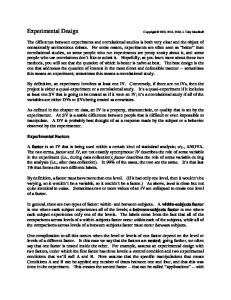
4 homogenous tasks (Table 2). The order of the first two induced values, $2 and $8, are reversed in the two sessions. In Session A, the 1st vote for each subject ($2 induced value) is combined with the 3rd vote ($5 induced value) from one other subject and the 4th vote ($8 induced value) of a third subject to determine the outcome of the group vote. The design for votes on programs with equal values of $2 or $8 is constructed similarly (Table 2). The extra four votes are not needed to complete the voting triplets. These additional votes are used to explore heterogeneous values for the $5 individuals. (NOTE: I have no idea what this last sentence means) Variations in the level of the uniform tax were set to favor detection of non-selfish behavior. The $7.50 tax is used to examine the behavior of the $8 voters, the $4.50 and $5.50 amounts are charged with measuring anomalies in subjects with a $5 induced value, while a $2.50 tax could detect non selfish or irrational behavior in the $2 value subjects. Figure 1 provides a comparison of voting in homogenous and heterogeneous conditions by subjects with a $2 induced value facing a $2.50 tax and those with a $8 induced values facing an tax of $7.50. When $2 subjects were in homogenous value groups ($2, $2, $2), 5.7% of subjects voted in favor of the program compared to 18.6% in the heterogeneous value case ($2, $5, $8). Using a t-test, this difference is statistically significant at the 1% level. For $8 value subjects facing a uniform tax of $7.50 on everyone, 86.4% vote in favor of the program when everyone stands to gain $8 while only 73.3% vote yes when the distribution of benefits is ($2, $5, $8). This difference is significant at the 3% level. In contrast, the behavior of the $5 value individuals is quite similar across homogeneous and heterogeneous setting, yielding no statistical differences at tax rates of either $4.50 or $5.50. In particular, for the higher cost of $5.50, 8.2% of subjects voted yes in the homogeneous treatment, while 12.2% votes yes in the heterogeneous treatment (p=0.505). For the lower cost

5 of $4.50, 92.3% votes yes in the homogeneous treatment, while 84.6% votes yes in the heterogeneous treatment (p=0.288). (Note: there is a disconnect here – I do not see any decision tasks in Table 2 with homo $5 distribution and costs of either $4.50 or $5.50. Most likely there is a typo for the 6th decision in both sessions) The detection of statistical differences in the behavior of the $2 and $8 subjects across value settings is an important indication that distributional considerations impact the utility of voters and their choices. In the heterogeneous value case, a tax of $7.50 would impose a loss of $2.50 on subjects with a $5 value and a loss of $5.50 on subjects with a $2 value. The results could indicate that subjects are concerned that they may impose losses on others (either all others, the “average” other subject or the worst of them). Similarly, the results of the $2 subjects would be consistent with those voters getting positive utility from the gains of others. Such a voting pattern is consistent with the conjecture made by Johansson et al (1996) in a stated preference study on the value of statistical life. They argued that pure altruism (also referred to as efficiency) implies that high value voters will lower their votes in consideration of voters who stand to gain less (or even lose). In the next section, we introduce a more effective mechanism and develop theoretical predictions of behavior for it. The mechanism will subsequently allow us to explore voting patterns in greater depth, and attempt to discriminate between alternative forms of social preferences motivating the subjects. 3. Theoretical Analysis and Testable Hypotheses In this section, we formally introduce the Random Price Voting Mechanism and develop theoretical predictions of bidding behavior for it. In order to efficiently measure the preferences of individuals in the context of a voting environment, a mechanism is needed that is transparent

6 and lends itself to single-shot elicitation of individuals’ maximum WTP and minimum WTA for parallel public goods. The mechanism proposed here meets these requirements by combining the private goods BDM mechanism with majority-rule voting. For private goods, the BDM mechanism (Becker et al. 1964) is incentive compatible and shows strong demand revealing properties (Irwin et al. 1998). The mechanism eliminates the incentives for strategic bidding as subjects only have to pay the randomly determined cost if their bid is greater than or equal to this cost, thereby making the true statement of maximum WTP (or minimum WTA) a dominant strategy. Laboratory experiments have further demonstrated the incentive compatibility and transparency of majority voting (see, for example, Plott and Levine 1978) and the binary discrete choice format has long been known to be incentive compatible (Farquharson 1969). These properties extend to the mechanism developed in this section. For ease of exposition, we present in some detail the derivations and theoretical predictions for the case where the game is played in the WTP for gains domain, and for the case where individuals have “social welfare” motives (Charness and Rabin, 2002). These results are readily extended to the other three Hicksian measures (WTP to avoid a loss and WTA a loss or forego a gain) and for all three other forms of preferences considered in this paper (Maximin, ERC and FS). Results for all those permutations are summarized in Table 3. Consider a situation where N individuals are asked to express the maximum amount of money they would be prepared to pay for an initiative defined simply by a known vector of values ∏ = (π1 , π 2 ,..., π N ) . The elements of the vector represent the individual gains to be received by the N individuals if the initiative is implemented, but the public program that is submitted to a “vote” has two components: 1) the induced values that would result, and 2) a transfer payment (C) from individuals to the implementing authority.

7 For the group to implement the program, a plurality (50%+1) of individuals must have expressed a WTP that exceeds a per-person cost C. As in the private BDM, this cost is randomly drawn from a distribution over the interval [0,C max ] after individuals have signaled their WTP. (In what follows, we develop theoretical predictions and implement the mechanism experimentally using a uniform distribution. We also refer to individual i’s signal as his “bid” and denote it with Bi ). If a majority of bids are greater than or equal to C, individual i receives a monetary payoff π i − C (which could be negative) to be added to an initial endowment Y. If the majority of bids is below C, no program is implemented and subjects retain their initial endowment. An individual has “social welfare” preferences if his utility is increasing (decreasing) in the gains (losses) of others. Thus, we posit that the total utility of individual i is given by ⎞ ⎛ U i = u ⎜ Y + π i − C + ∑ α i ⋅ (π j − C) ⎟ , where α i ≥ 0 is a parameter indicating the intensity with ⎠ ⎝ j≠i

(

)

which the utility of individual i is affected by the gains and losses of others. The term in the summation allows for the fact that subjects may have positive preferences for the benefits that others receive from the implementation of the program. Heterogeneity across subjects is admitted through individual values of α i . In particular, a purely selfish individual is characterized by α i = 0 . To compute the Bayesian Nash Equilibrium bid of individual i, it is useful to rank order the bids of all n-1 other individuals. Define Bm as the bid that ranks as the Integer ((n + 1) / 2)th largest of those bids (for n=3 this is the smallest of the other two bids). It is also useful to define Bk as the Round ((n − 1) / 2) th largest bid (for n=3, this identifies the largest of the other two bids).

8 The interval [Bm , Bk ] defines the range over which the bid of voter i makes this individual have a marginal influence on the outcome of the game (in a probabilistic sense, it makes him the median voter). To see this, consider i’s expected utility (where B-i are the bids from all other individuals in the voting group):

(

Bm

⎛

) ∫ p(C)U ⎜⎝ Y + π

EU i Bi , B− i =

0

i

⎞ − C + ∑ α i ⋅ (π j − C) ⎟ dC ⎠ j≠i

(

)

⎛ + ∫ p(C)U ⎜ Y + π i − C + ∑ α i ⋅ (π j − C) ⎝ j≠i Bm Bi

Bk

(

()

+ ∫ p(C)U Y dC + Bi

Cmax

∫

⎞

)⎟⎠ dC

(1)

()

p(C)U Y dC

Bk

The first term denotes the expected utility conditional on the randomly drawn cost being below Bm. In this case, i’s bid is completely irrelevant to the outcome since a sufficient number of other voters exist who are willing to pay at least the drawn cost C to implement the program. The second and third terms cover the interval over which the bid of individual i will have a marginal effect on the probability that the program will be implemented. Here, Bi is effectively the median bid (again, in a stochastic sense). By increasing his bid, individual i increases the upper bound of the range of costs that a plurality of voters is prepared to pay (second term), and decreases the range over which the project is not implemented (third term). The last term is the interval for which no matter how high individual i’s bid is, the program will not be implemented since strictly fewer than half of the other players are prepared to pay a cost in that interval. In searching for equilibrium bidding strategies, we limit our attention to the family of affine strategies. Individual i conjectures that individuals m and k choose bids of the form

⎛ ⎞ Bm = γ m ⎜ π m + ∑ α m π j ⎟ j≠m ⎝ ⎠

(2)

9 and

⎛ ⎞ Bk = γ k ⎜ π k + ∑ α k π j ⎟ . j≠k ⎝ ⎠

(3)

Where γ k and γ m are positive constants, the exact value of which is defined by the equilibrium solution below. Substituting these expressions in Equation 1 and maximizing by choosing Bi yields the first order condition: ⎧⎪ ⎛ ⎞ ⎫⎪ p ( Bi ) ⎨ −U (Y ) + U ⎜ Y + π i − Bi + ∑ (α i ⋅ (π j − Bi ) ) ⎟ ⎬ = 0 . j ≠i ⎝ ⎠ ⎭⎪ ⎩⎪

(4)

This equation has a degenerate solution p ( Bi ) = 0 (where Bi is set equal to the lower support of the cost distribution). Assuming concavity of the utility function, there is also an interior maximum whereby individual i chooses his bid so as to equate utility under the two alternative states of the world (the program is funded or it is not). This optimal bid is given by:

B = * i

π i + ∑ αi π j j ≠i

1 + ( N − 1)α i

.

(5)

This optimal strategy has the same form as the priors of individual i regarding the bidding strategies of individuals m (Equation 2) and k (Equation 3) if one sets γ i = 1 (1 + ( N − 1)α i ) . Thus, if all N players adopt the linear conjecture and bid accordingly, their conjectures are proved correct and (5) constitutes a symmetric Bayesian Nash Equilibrium. Note that an individual’s optimal bid does not require knowledge of the α j ’s of other individual. A number of characteristics lead directly to testable behavioral predictions. 1) The standard individual BDM is a special case that can be recovered from the voting mechanism. To see this, set N=1 in Equation 5. This yields the well-known BDM incentive compatibility result: Bi* = π i .

10 2) The model predicts that if the payoffs are identical across subjects ( π j = π i ∀j ), the optimal strategy is for individual i to bid an amount equal to his own personal payoff

(Bi* = π i ) . In this case, the individual sensibly recognizes that if he were to bid above the common value, the resulting increase in the probability that the program will be funded is, in equilibrium, simply increasing the possibility that the program will be implemented at a cost exceeding value. This could result in a net loss for all subjects, making bids above value irrational. Similar reasoning leads to the conclusion that bidding below the common value is also sub-optimal individually and collectively. 3) Any change in the vector that increases total gains for the group draws an increase in the optimal individual bid. The two relevant derivatives establishing this result ∂Bi* αi = >0 ∂π j 1 + ( N − 1)α i

(6)

∂Bi* = 1. ∂π i

(7)

and

4) By extension, increasing (decreasing) the sum of other’s payoffs increases (decreases) the optimal bid. For our purposes, this implies that individual i should increase (decrease) his bid when going from a situation where π i = π j = π ∀j to one where all payoffs other than his are increased (decreased). Similarly, changes in the payoffs of others (only) that leave the sum of payoffs unchanged (that preserves the mean of the payoffs of others) would have no impact on Bi*. These predictions are summarized in Table 3. 3.1 WTA and Losses

11 The theory can easily be reinterpreted to describe the optimal bidding strategy for an individual expressing his minimum willingness to accept (WTA) compensation to forego gains. In this case, C represents the randomly determined compensation to be paid to abandon a program defined by the vector ∏ . Bi denotes the smallest amount that individual i would accept. If a majority of bids are less than or equal to C, compensation C is paid, but the gains ∏ that

⎛ ⎞ were to be received are not. Thus, the utility level is U ⎜ Y + C + α i ∑ C ⎟ . Otherwise, the j ≠i ⎝ ⎠ ⎛ ⎞ program the program is not implemented and utility is U ⎜ Y + π i + α i ∑ π j ⎟ . j ≠i ⎝ ⎠ Re-deriving the optimal bid strategy yields exactly the result of Equation 5, and thus, all theoretical predictions follow. Some care should be taken, however, in interpreting the results. Here, the vector ∏ represents individual opportunity costs of implementing the compensation program. Thus, an increase in this opportunity cost (to any player) implies a decrease in the social value of the compensation offer and thus an increase in the minimum acceptable level of compensation required by voters. Similar exercises can be conducted to derive the optimal strategy for the Willingness to Accept compensation for a program that imposes a loss and for the Willingness to Pay for a program that eliminates such a loss. Once again, care must be exercised to ensure proper interpretation of the theoretical predictions, but algebraically, Equation 5 is exactly replicated in both cases and the same comparative static results follow. 3.2 Alternative Forms of Other-Regarding Preferences Similar approaches can be followed to analyze the optimal bidding strategies under alternative structures for other-regarding preferences. Of particular interest in this paper are three other utility functions that our experimental data will allow us to compare against the social

12 efficiency alternative. They are the maximin utility (Charness and Rabin, 2002) (MM), a version of Bolton and Ockenfels (2000) (ERC) theory of equity, and Fehr and Schmidt (1998) (FS) inequity aversion preferences. If an individual has maximin preferences, his utility depends on his own payoff as well as on the (potential) gains or losses of the individual who stands to gain the least (lose the most). Someone with preferences for equity gets disutility from distributions of payoffs that exhibit deviations about the mean. In ERC preferences, one’s disutility stems directly from a comparison between one’s payoff and the mean of everyone’s payoff. This generates a situation where there is no disutility if one stands to obtain exactly the mean payoff. In contrast, FS preferences postulate that any inequity in a distribution generates personal disutility. For brevity, we forego the detailed exposition of the derivations for the three additional utility formulations and four Hicksian measures. Table 3 provides a summary of behavioral predictions. Table 3 must be interpreted with some care. The basic formulation (Column 2) is given for WTP for Gains where π > 0 and C>0. Thus, the optimal bid (Column 3) is a positive amount and the behavioral prediction (Column 4) is readily interpreted. For the other cases, the optimal bid formula and the behavioral predictions are written for the absolute values of π i ,

π j and C and therefore positive values for Bi* . Take the following example with three individuals and a homogenous distribution of payoffs ($2, $2, $2). These could be gains or losses depending on the context. In all cases, however, the predicted bid is Bi* = $2 for all players. This optimal bid represents alternatively the maximum WTP to secure a gain of $2 or to avoid a loss of $2; or the minimum WTA a loss or forego a gain. For heterogeneous distributions, consider the vector ($2, $5, $8) as an example and lets now review each of the preferences’ predictions.

13 3.2.1 Social Welfare For the social welfare preferences formulation, an individual with a $2 induced value is predicted to bid an amount greater than $2, in the WTP cases. This is reasonable, since the individual values the high benefits to others and is thus prepared to incur a personal cost to increase the probability that the program will be implemented. For the same reason, the minimum amount of compensation the $2 individual requires is more than the amount he risks to lose or forego because this also increases the probability that the program will be implemented and that the others who have more at stake than he does will benefit from the program. Thus, regardless of the scenario, we recognize the “smallest π ” as the smallest absolute induced value, be it a gain or a loss). 3.2.2 Maximin In the case of maximin preferences, it is necessary to identify who in the group is potentially made worse off by the implementation of the program. In WTP cases, the person who potentially gains the least (loses the most) from the program is the one with the smallest induced value ( π w = $2 in our example). This is true regardless of whether the WTP is for a gain of $2 or to avoid a loss of $2. The program has little benefits for this individuals and he could even have to pay a hefty price C for it. The prediction is that this person will bid $2 and others, who have a larger stake in the program will bid less than there induced value in order to reduce the probability that a loss will be imposed on the $2 individual. In WTA scenarios, the individual with a high absolute induced value is the one potentially made the worst off by the program. If the program is implemented, they have to forego the largest gain or suffer the largest lost. Thus, for our example, π w = $8 in the WTA cases. The prediction is then that those with lower induced values will set Bi* > π i since doing so

14 in a WTA scenario, in an effort to reduce the probability of imposing welfare costs on the $8 individual. 3.2.3 ERC Preferences Individuals with equity preferences also present a particular pattern of optimal bidding. Any program that results in an inequitable distribution of payoffs produces individual disutility for all subjects who do not receive a payoff equal to the mean. In other words, all programs with heterogeneous distributions of induced values will generate disutility for those who do not have a payoff equal to the mean. In the gains domain, individuals will therefore be willing to pay less than their private value for a program that provides additional income, they would also require a smaller amount of compensation to forego such gains since foregoing the personal gains also relieves them of the disutility of the inequitable distribution. The opposite is true in the losses domain. Individuals will require more than their private value in compensation to accept a loss since compensation must also cover the inequity cost resulting from of the program. Similarly, individuals other than ones with a mean π i would be willing to pay more than their value to avoid a loss, since once again, the heterogeneity of losses entails additional disutility. 3.2.4 FS Preferences With FS preferences, all individuals (even one with a payoff equal to the mean) gets disutility from a heterogeneous distribution. What drives the disutility is a direct comparison of one’s payoff with that of other individuals rather than with the mean payoff. A second difference with ERC comes from the fact that FS preferences allow for different valuations of positive and negative differences between individual payoffs. Fehr and Schmidt postulate that individuals are less affected by differences in their favor than by situations where they are the poor party in the

15 comparison (a situation that would be characterized by α i ≥ β i ). It is readily deduced that all individuals in any game with heterogeneous distributions will be willing to pay less than their induced value for gains and willing to accept less than induced value to forego a gain unequal to that of others. By the same logic, all individuals will be willing to pay more than induced value to avoid a loss, and require greater compensation to accept a loss that also carries a disutility cost from inequity. 4. Experimental Design

To test the theories outlined above, an additional 276 subjects volunteered for the experiments and were recruited from a variety of undergraduate economics courses. Each session consisted of either two WTP experiments: WTP-Gains and WTP-Losses (n=138) or two WTA experiments: WTA-Gains and WTP-Losses (n=138), thereby representing all four welfare settings. All sessions consisted of four parts; an example session is as follows: Part A:

WTP-Losses, low-incentive private BDM rounds where the cost is determined and payoffs calculated at the end of each round.

Part B:

WTP-Losses, high-incentive private and public RPVM treatments where the treatment and cost which result in earnings is determined at the end of the experiment.

Part C:

WTP-Gains, low-incentive private BDM rounds where the cost is determined and payoffs calculated at the end of each round.

Part D:

WTP-Gains, high-incentive private and public RPVM treatments where the treatment and cost which result in earnings is determined at the end of the experiment.

To control for potential order effects, whether the two gains scenarios were encountered first varied across sessions. Further, Part B and Part D varied the order of the treatments with respect to induced gains or losses, the amount of the induced values, voting group size, and the distribution of values among group members. In public RPVM treatments subjects were

16 provided complete information about the payoff amounts of the other subjects. To prevent deterioration of other-regarding behavior that can occur in voluntary public good mechanisms (Davis and Holt 1993), subjects submitted bids for the public treatments (Part B and Part D) without feedback. At the end of the experiment one of the nine RPVM programs was implemented from both Part B and Part D by having the subjects draw from a bag of marked poker chips. The exchange rate for Part A and Part C was fifteen experimental dollars for one US dollar, while the exchange rate for Part B and Part D was one experimental dollar for one US dollar. The experiment lasted approximately two hours and the average payoff was $35. Subjects received written instructions (Appendix B). As part of the verbal protocol, they were permitted to ask questions at the beginning of each part of the experiment. The instructions used language parallel to that found in surveys for referendum voting settings (Boyle 2003). (Note: the Carson et al. working paper was a weird cite!) The WTP instructions directed each subject to vote whether to fund a program by submitting a bid that represented the “highest amount that you would pay and still vote for the program.” The WTA instructions directed each subject to vote whether to implement a program by submitting an offer that represents the “lowest amount of compensation that you would accept and still vote against the program.” Each subject was seated at an individual computer equipped with a privacy shield. Subjects were assigned into voting groups of varying size of either one or three. For the groups of three, the administrators announced the groups and asked each group member to raise their hand so that they could be identified by other members of their group. This ensured that subjects were aware of who was in their voting group for all treatments. No communication was allowed. For simplicity, consider the WTP-Gains experiment. In each round, subjects started with an initial balance of $10 and were assigned an induced value ($1, $2, $4, $5, $6, $8 or $9).

17 Subjects then decided how much to bid ranging from zero to the entire initial balance. After the subjects submitted their bids, the cost for the program was determined. This cost was determined by using a random numbers table with values from zero to nine. The first random number from the table represented the dollars amount, the second number the dimes amount, and the third number the pennies amount. For example, if the first random number was a four, the second was a nine, and the third a four, the determined cost would have been $4.94. Consequently, the cost was uniformly distributed between $0.00 and $9.99 with discrete intervals of $0.01. The RPVM operated in much the same way as the traditional private good BDM mechanism with a couple of key differences. In the RPVM a majority of votes (based on the amount of each individual’s bid) determines whether the program is funded. Consequently, treatments with group size of one are identical to the private good BDM as each subject’s bid constitutes a majority. In WTP-Gain treatments, if the majority of the bids are greater than or equal to the randomly determined cost, then the program is funded. In this case, all of the subjects in the voting group receive their personal payoff amount in addition to the initial balance, but also have to pay the determined cost. If the majority of bids are less than the randomly determined cost, then the program is not funded. In this case, all of the subjects in the voting group neither receive their personal payoff amount nor pay the cost, and thus, the subjects receive only their initial balance. For each welfare treatment, the majority of the public good treatments with heterogeneous values were conducted with symmetric distributions – i.e. $2, $5, $8 (93 subjects each). To help identify the alternative social welfare measures, experiments were also conducted that had public good treatments with heterogeneous values with asymmetric distributions – i.e. $4, $5, $9 (45 subjects each).

18 In the private good treatments, a subject’s optimal strategy is to submit a bid equal to her induced value. Due to the discrete costs, another optimal strategy is to submit a bid which is one penny less than the induced value. For the voting groups of three subjects, the majority rule introduced a coercive tax element, because if a majority of the group submitted bids greater than or equal to the randomly determined price, then everyone had to pay the price regardless of their individual bids. This coercive element is highlighted in the heterogeneous treatments where majority rule can force a low value subject to pay a cost that was greater than their value or could deny a high value subject benefits that he would have otherwise obtained in a private treatment. For the WTP-Losses experiments if a majority of the bids is less than the random cost, the program is not funded. Consequently, all group members have their personal loss amount ($1, -$2, -$4, -$5, -$6, -$8 or -$9) deducted from their initial balance of $10. If the majority of bids are greater than or equal to the determined cost, the program is funded and all voting group members have to pay the determined cost from their initial balance of $10 but do not have the personal loss amount deduced. For WTP-Losses, the same logic holds as the majority rule could force a low value subject to pay a higher cost then their induced value and the high value subject may be denied the opportunity of paying a cost lower than their induced value. The logic of how the vote creates a coercive tax element in for both the induced gains and induced losses treatments is identical in the WTA-Gains and WTA-Losses experiments. For the WTA experiments, the subjects submit offers which represented the lowest amount of compensation they would accept where the optimal offers are either the induced value or one penny above it. The induced gains and losses are the same as the WTP setting and the possible compensation again ranges from $0.00 to $9.99. To avoid income effects, the initial balance is $5 which made the expected earnings in the WTA setting equivalent to the WTP

19 setting. In WTA-Gains, an offer is the lowest amount a subject would accept to vote against the program which otherwise would provide the subject a gain. If the majority of the offers are less than or equal to the random compensation, then the program is not implemented and all voting group members receive the compensation in addition to their initial balance. If the majority of the offers re greater than the random compensation, the program is implemented and the group members receive their personal payoff amount in addition to their initial balance. In contrast, in WTA-Losses, an offer represents the lowest amount a subject would accept to vote in favor of the program, which forces the subject to pay the induced loss if funded. Therefore, if the majority of offers are less than or equal to the random compensation, the program is implemented and all group members receive the compensation and the initial balance but have to pay their induced losses. If the majority of the offers are greater than the random compensation, the program is not implemented and all group members keep their initial balance. 5. Results

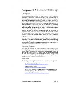
Similar to other studies using the BDM mechanism (Boyce et al. 1992; Irwin et al. 1998), the goal of the low-incentive rounds was to give subjects an opportunity to gain experience with the mechanism before introducing additional complexities to the decision environment. Repeated low incentive private BDM rounds provided subjects an opportunity to receive feedback on how their bids and offers affected their payoff. Over ten practice rounds, subjects bids/offers converged towards induced value, starting at $0.69 above induced value in the first round and declining by 70% to only $0.21 above induced value in the tenth round (Figure 1). For the WTP practice rounds, the average bid decreased from $0.67 to $0.25 above induced value (an improvement of 63%). For the WTA practice rounds, the average bid decreased from $0.72 to $0.17 above induced value (an improvement of 76%). Overall, while learning was obviously

20 taking place during practice rounds, by the last practice round subjects were submitting bids that were statistically indistinguishable from their induced values in all four welfare settings. (Note that we eventually will need to state how these tests were conducted)

5.1 Comparing RPVM with Dichotomous Choice Voting In the public good treatments with symmetric, heterogeneous value distributions, the resulting pattern of bids appears similar to what is observed earlier in the case of dichotomous choice voting. For example in the RPVM, 23.7% of subjects with a $2 value indicated that they would pay at least $2.50 for a program that had benefits that were distributed heterogeneously ($2, $5, $8). This percentage is statistically indistinguishable from the 18.6% of subjects who voted yes in the similar dichotomous choice voting setting (Table 4). In fact, none of the twelve dichotomous choice voting settings yielded results that are statistically different than the results of the RPVM. This suggests that RPVM elicits values that are consistent with dichotomous choice voting and establishes the RPVM as an efficient alternative from which to examine anomalies in voting.

5.2 General Voting Patterns The experiments yield 76 unique treatments under high-incentive conditions, where a treatment is defined by a specific welfare setting (e.g. WTP-gains), the subject’s induced value, and the distribution of other players’ values (if any). To facilitate comparisons between bidding behavior and induced values, we pool the data from all high-incentive rounds and regress individual bids on 76 indicator variables to produce estimates of the average bid in each treatment. As each individual produces multiple observations, we estimate robust standard errors

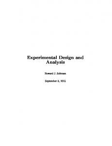
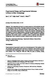
21 adjusted for clustering at the individual level. As all decisions from the individual are made without feedback, there are no controls for learning behavior. Table 5 and Table 6 present the treatment-specific mean bids for the gains and loss settings, respectively, in both WTP and WTA settings. Estimates that are statistically different than induced value at the 5% level are italicized. Inspection of the results shows several patterns. First, as expected, eleven of the twelve bids/offers in the private settings are statistically indistinguishable from induced value. This result can be seen in Figure 3, where the private values line up nearly perfectly with the 45 degree line representing the induced values. Second, all of the bids/offers in the twenty-eight homogeneous treatments are not statistically different than induced value. Again this pattern can be observed in Figure 3. Third, a different pattern clearly emerges in the treatments with heterogeneous distribution of values. In these cases, the low-value subjects raise their bids/offers and the high-value subjects lower their bids/offers. In the eight treatments that had the lowestvalue subject have an induced value that was more than a dollar less than the middle-value subject (subjects with induced gains and losses of $1 and $2), subjects significantly raised their WTP/WTA in seven of the eight treatments. Likewise, when the highest-value subjects had an induced value that was more than a dollar higher than the middle-value subject ($8 and $9 values), subjects significantly lowered their WTP/WTA in seven of the eight treatments. As can been seen in Figure 3, a clear pattern emerges that relative to the 45 degree line which represents the induced values, in heterogeneous value settings the worst-off subjects raise their bids/offers in a voting context and the best-off subjects lower their bids/offers. In heterogeneous treatments there is not a systematic divergence from induced values for middle-value ($5) subjects. Symmetric distributions produce bids that are roughly equal with value, although in one of four cases there is a statistical difference. In asymmetric distribution

22 treatments, there is a weak tendency for middle-value subjects to bid to bid below value when their value is above average (i.e. the $1, $5, $6 distribution) and a weak tendency to bid average value when their value is below average (i.e. the $4, $5, $9 distribution). For heterogeneous treatments with asymmetric distributions, all of the means were above induced value for the low-value subjects and lower than induced value for the high-value subjects. However, many of these differences were not statistically different than zero. In particular, statistical differences tend to occur when there is a large spread between the value of the high (low) value subject and the middle and low-value subjects. When the high (low) value subject has a value close to the middle-value subject, statistical differences generally are not observed.

5.3 Performance of Social Preference Theories In the final part of our analysis we investigate the extent to which the four social choice theories discussed in Section 3 may explain observed bidding behavior. The econometric analysis is loosely based on that of Engelmann and Strobel (2004). A casual comparison between the behavioral predictions presented in Table 3 and the results of tests of mean bids against induced values suggest that the data is consistent with social efficiency considerations. At least for symmetric value distributions we found clear indications that low-value subjects bid above value and low value subjects bid below value. This also could be partially explained by maximin preferences. The two inequality aversion theories do not appear to organize the data well as there does not appear to be systematic differences in bidding behavior between gains and loss scenarios. More generally, there do not seem to be systematic differences across the four welfare scenarios.

23 To more formally test the social welfare theories we regress individual bids in public good treatments on measures that correspond with the theory-specific components of the utility function (Table 3), as well as a variable that corresponds with self-interest. Variable definitions are presented in Table 7. Note that while we pool data from all four welfare scenarios for our regressions, the implied coefficient restrictions are justified in all cases by statistical tests. Similar to the previous regression, we generically allow for heteroscedastic errors and correlation between responses through the use of a robust covariance estimator adjusted for clustering at the individual-level. In order to accommodate bids and losses into the same model, the negative of the bid is used in loss treatments. This produces consistent expected coefficient signs (in particular the expected signs on all variables is positive) for all four welfare scenarios. Table 8 presents several models. We first estimate a “Kitchen Sink” model (Model I) that allows the possibility that all four social welfare motives – Efficiency, Maximin, ERC, FSstrict – along with self interest (Self) explain average bidding behavior. Such a model is consistent with the notion that motives across individuals may be heterogeneous and two or more motives may explain the behavior of the representative individual. Self interest and efficiency are the only statistically significant motives. Given that the social preference measures are closely related in the sense that they predict similar behavior in instances, it is not surprising that these covariates are highly collinear, as indicated by very high variance inflation factors (VIFs), which average almost 90. In lieu of this collinearity we also estimate theory-specific models (Models II – V) whereby bids are independently regressed on Self and each social preference variable. For the FS model, the FSstrict measure is separated into its disadvantageous (FSα) and advantageous (FSβ) inequality components to allow for separate effects. When investigated in isolation, only efficiency and maximin measures are statistically significant and have the correct coefficient

24 sign. Both FS measures are statistically significant, but the disadvantageous measure has the opposite sign. Given the previous statistical tests of bid versus value, this is not surprising as the theory suggests that high and low-value individuals would adjust their bid relative to induced value in the same direction whereas in actuality high and low-value individuals tend to bid relative to induced value in opposite directions. If the measure FSstrict were instead included it would be statistically insignificant, similar to the ERC measure. Overall, the inequality aversion theories appear to explain little about average behavior. In order to better distinguish between the relative importance of efficiency and maximin preferences, we included both these measures (along with Self) in a regression. Similar to the Kitchen Sink model, efficiency is a statistically significant factor whereas maximin is not. Looking closer at the predictions in Table 3, if maximin preferences were driving results one would expect that, say, in the heterogeneous treatments with a symmetric distribution that middle-value WTP (WTA) respondents would bid below (above) value. This is not consistent with behavior. Further, we should see worst-off individuals bidding at value, but it is clear that these individuals have concerns for best-off persons. In sum, while there is some evidence that maximin considerations may drive bidding behavior in these experiments, preferences for efficiency seem most consistent with the data and explain a wider range of observed bidding tendencies.

6. Conclusion

The evidence presented in this paper suggests that the public good version of the BDM mechanism, which utilizes voting in a coercive tax setting, is demand revealing. In addition, no WTP/WTA discrepancies are evident. However, the result that the participants with high induced

25 gains (low induced gains) tend to understate (overstate) their WTP and WTA relative to induced value (this pattern is mirrored in the induced loss treatments) is most succinctly explained by social concerns for efficiency (pure altruism). Equity or relative rank concerns do not seem to add much explanatory power in this setting utilizing induced values and undergraduate business majors. Clearly in other contextual settings such as dictator games, equity plays a major role. It should be noted that our findings are consistent with a conjecture made by Johannesson et al. (1996), who argued that the coercive nature of voting and taxation also raises the possibility, that some people will vote “no” on a project that would provide them private net benefits, narrowly defined, because they desire not to impose costs on others for whom costs exceed the benefits, and attributed this possibility to pure altruism. Their evidence was obtained from hypothetical survey questions about voting for or against safety programs. The experiments presented in this paper represent a potential starting point from which these issues can be examined further. Extensions of the RPVM include changes in voting group size when values are heterogeneously distributed, changes in the distributions of the heterogeneous treatments, the use of commodities, and the application of the mechanism to examine how various behavioral anomalies respond to public good settings.

26 References

Andreoni, J. 1990. Impure Altruism and Donations to Public Goods: A Theory of Warm Glow Giving. The Economic Journal 100(401): 464-477. Andreoni, J. 1995. Cooperation in Public Goods Experiments: Kindness or Confusion? American Economic Review 85: 891-904. Archibald and Davidson. 1976. Non-Paternalism and the Basic Theorems of Welfare Economics. Canadian Journal of Economics. 9: 492-507. Becker, G.M., M.H. DeGroot, and J. Marshack. 1964. Measuring Utility by a Single-Response Sequential Method. Behavioral Science (July): 226-32. Bergstrom, T. C., 1982. “When is a Man’s Life Worth More then His Human Capital?” in JonesLee, M. W. (ed.), The Value of Life and Safety, North-Holland, Amsterdam. Bolton, Gary E., and Axel Ockenfels, 2000, "ERC: A Theory of Equity, Reciprocity, and Competition." American Economic Review, vol. 90, issue 1, pages 166-193 Boyce, R.R., T.C. Brown, G.H. McClelland, W.D. Schulze, and G.L. Peterson. 1992. An Experimental Examination of Intrinsic Environmental Values. American Economic Review 82(5): 1366-1372. Boyle, Kevin J. 2003. Contingent Valuation in Practice. In A Primer on Nonmarket Valuation, Patricia A. Champ, Kevin J. Boyle and Thomas C. Brown (eds.). Dordrecht, The Netherlands: Kluwer Academic Publishers. Charness, Gary and Matthew Rabin. 2002. Understanding Social Preferences with Simple Tests. The Quarterly Journal of Economics. 117(3): 817-869. Chilton, S.M. and W.G. Hutchinson. 1999. Some Further Implications of Incorporating the Warm Glow of Giving into Welfare Measures: A Comment on the Use of Donation Mechanisms by Champ et al. Journal of Environmental Economics and Management 37(2): 202-209. Cummings, R.G., S. Elliott, G.W. Harrison, and J. Murphy. 1997. Are Hypothetical Referenda Incentive Compatible? Journal of Political Economy 105(3): 609-62 Davis, Douglas D. and Charles A. Holt. 1993. Experimental Economics. Princeton, New Jersey: Princeton University Press. Engelmann, Dirk and Strobel, Martin. 2004. "Inequality Aversion, Efficiency, and Maximin Preferences in Simple Distribution Experiments." American Economic Review 94(4): 857-869.

27 Farquharson, R. 1969. Theory of Voting. New Haven: Yale University Press. Ferarro, P. J., D. Rondeau, and G. L Poe, 2003. Detecting ORB with Virtual Players. Journal of Economic Behavior and Organization 51:99-109. Fehr, Ernst and Schmidt, Klaus M. "Theories of Fairness and Reciprocity - Evidence and Economic Applications." CEPR Discussion Papers 2703, C.E.P.R. Discussion Papers, February 2001. Flores, N. E., 2002. “Non-Paternalistic Altruism and Welfare Economics”, Journal of Public Economics, 83:293-305. Goeree, J. K., C. A. Holt, and S. K. Laury. 1999. Altruism and Noisy Behavior in One-Shot Public Goods Experiments. Manuscript, Department of Economics, University of Virginia. Hanemann, W.M.. 1994. Valuing the Environment through Contingent Valuation. Journal of Economic Perspectives 8(4): 19-43. Horowitz, J.K. and K.E. McConnell. 2002. A Review of WTA / WTP Studies. Journal of Environmental Economics and Management (44): 426-447 Irwin, J.R., G.H. McClelland, M. McKee, W.D. Schulze, and NE. Norden. 1998. Payoff Dominance vs. Cognitive Transparency in Decision Marking. Economic Inquiry 36(2): 272-285. Johannesson, M., P-O. Johansson, and R.M. O’Conor. 1996. The Value of Private Safety Versus the Value of Public Safety. Journal of Risk and Uncertainty (13): 263-275. Johannsson, P-O, 1993. Cost Benefit Analysis of Environmental Change, Cambridge University Press, Cambridge, UK. Johannsson, P-O, 1994. “Altruism and the Value of Statistical Life: Empirical Implications”, Journal of Health Economics, 13:111-118. Jones-Lee, M. W., 1991. “Altruism and the Value of Other People’s Safety”, Journal of Risk and Uncertainty, 4: 213-219. Jones-Lee, M. W., 1992. “Paternalistic Altruism and the Value of Statistical Life”, The Economic Journal 102: 80-90. Madariaga, B. and K.E. McConnell. 1987. Exploring Existence Value. Water Resources Research 23(5): 936-942.

28 Milgrom, P. R., 1993. “Is Sympathy an Economic Value? Philosophy, Economics and the Contingent Valuation Method”, in Hausman, J. A. (ed.), Contingent Valuation: A Critical Assessment, North-Holland, Amsterdam. Palfrey, T. P. and J. E. Prisbey. 1997. Anomalous Behavior in Public Goods Experiments: How Much and Why? American Economic Review 87: 829-846. Poe, G.L., J.E. Clark, D. Rondeau and W.D. Schulze. 2002. Provision Point Mechanism and Field Validity Tests of Contingent Valuation. Environmental and Resource Economics 23: 105-13. Plott, C.R. and M. Levine. 1978. A Model of Agenda Influence on Committee Decisions. American Economics Review (68): 147-160. Rondeau, D., G.L. Poe, and W.D. Schulze. 2005. “VCM or PPM? A Comparison of the Performance of Two Voluntary Public Goods Mechanisms.” Journal of Public Economics 89:1581-1592. Rondeau, D., G.L. Poe, and W.D. Schulze. 1999. Voluntary Revelation of the Demand for Public Goods Using a Provision Point Mechanism. Journal of Public Economics. 72: 455-470. Schulze, W.D., G.L. Poe, I. Bateman, and D. Rondeau. 2002. Is the Scope Test Meaningful In the Presence of Other Regarding Behavior? in J.A. List and A. de Zeeuw, eds. Recent Advances in Environmental Economics., Edward Elgar Publisher.

29 APPENDIX A: DICHOTOMOUS CHOICE INSTRUCTIONS Instructions This is an experiment in the economics of decision making. In the course of the experiment, you will have opportunities to earn money. Any money earned during this experiment is yours to keep. It is therefore important that you read these instructions carefully. Please do not communicate with other participants during the experiment. In today’s experiment, you will be asked to vote for or against six different programs. In this experiment, a program is simply a distribution of money. As you will see, your vote will help determine whether or not the program is funded. The procedures that will be followed are the same for all programs. However, each program and vote is independent from the other. Therefore, your vote in one program will not affect the results for other programs. Only one of the six programs will actually be implemented and result in cash earnings. At the conclusion of the experiment, we will randomly determine which of the programs will generate cash earnings by drawing from a bag containing six chips lettered A through F which correspond to each program. For each program, the experiment proceeds as follows: For each of the programs, you will be part of a group of three voters. First, you and every other member of your group will receive an initial balance of $10.00. You will then be informed of your personal payoff amount for this program. Your personal payoff amount is the amount of money that you will receive if the program is funded. Your personal payoff amount will vary during the course of the experiment. The possible amounts are $2.00, $5.00, and $8.00. The payoff amounts that the other voters in your group would receive if the program is funded are indicated on your computer spreadsheet. Your spreadsheet also will inform you of the per person cost of the program. This is the cost that you and everyone else in your group would have to pay if the program is funded. You will then be asked to vote for (“Yes”) or against (“No”) this program. You will submit your vote by clicking the “Submit” button. For each program, there are two possible outcomes: The program is NOT FUNDED: The program is not funded if a majority of votes from your group are “No.” In this case, neither you nor any other member of your group will receive a personal payoff amount and no one will pay the cost. Therefore, your cash earnings for this part of the experiment would simply be your initial balance of $10.00. The program is FUNDED: The program is funded if a majority of votes from your group are “Yes.” In this case, you will receive your personal payoff amount in addition to your initial balance. However, you will also have to pay the per person cost. Every other member of your group will also receive their personal payoff amount and they will also have to pay the same per person cost. Therefore, your cash earnings would be your initial balance ($10.00), plus your personal payoff amount, minus the per person cost. At the conclusion of the experiment, a volunteer subject will draw which of the six programs will be implemented to determine your cash payoff. Upon notification by the administrator, please click the “Update Results” button.

Table 1: Dichotomous Choice Experiment – Heterogeneous Value Design (n=86).

Session A Treatment 1st 2nd

Initial Endowment $10 $10

Own Reward $2 $8

Others Rewards $5, $8 $2, $5

Uniform Cost $2.50 $7.50

Expected Earnings $9.50 $10

3rd 4th 5th 6th

$10 $10 $10 $10

$5 $8 $2 $5

$2, $8 $2, $5 $5, $8 $2, $8

$2.50 $2.50 $7.50 $7.50

$12.50 $15.50 $10 $10

Treatment 1st 2nd

Initial Endowment $10 $10

Own Reward $8 $2

Others Rewards $2, $5 $5, $8

Uniform Cost $7.50 $2.50

Expected Earnings $10 $9.50

3rd 4th 5th 6th

$10 $10 $10 $10

$5 $2 $8 $5

$2, $8 $5, $8 $2, $5 $2, $8

$7.50 $7.50 $2.50 $2.50

$10 $10 $15.50 $12.50

Session B

31 Table 2: Dichotomous Choice Experiment – Homogeneous Value Design (n=88)

Session A Treatment 1st 2nd

Initial Endowment $10 $10

Own Reward $2 $8

Others Rewards $2, $2 $8, $8

Uniform Cost $2.50 $7.50

Expected Earnings $10 $10.50

3rd 4th 5th 6th

$10 $10 $10 $10

$2 $5 $8 $5

$5, $8 $2, $8 $2, $5 $5, $5

$4.50 $4.50 $4.50 $5.00

$7.50 $10 $13.50 $10

Treatment 1st 2nd

Initial Endowment $10 $10

Own Reward $8 $2

Others Rewards $8, $8 $2, $2

Uniform Cost $7.50 $2.50

Expected Earnings $10.50 $10

3rd 4th 5th 6th

$10 $10 $10 $10

$8 $5 $2 $5

$2, $5 $2, $8 $5, $8 $5, $5

$5.50 $5.50 $5.50 $5.00

$10 $10 $10 $10

Session B

32 Table 3. Summary of Theoretical Predictions.

Preference Other Regarding Component Type of the Utility Function

Optimal Bid

Behavioral Predictions

Social Efficiency

+α i ∑ (π j − C )

π i + ∑αi π j

N=1 ⇒ Bi* = π i Homogeneous ⇒ Bi* = π i Heterogeneous Mean π : Bi* = π i Smallest π : Bi* > π i Highest π : Bi* < π i

Maximin

+α i (π w − C )

j ≠i

j ≠i

1 + ( N − 1)α i

π i + α iπ w 1 + αi

N=1 ⇒ Bi* = π i Homogeneous ⇒ Bi* = π i Heterogeneous If π i = π w ⇒ Bi* = π i If π i > π w ⇒ Bi* < π i (WTP) If π i < π w ⇒ Bi* > π i (WTA)

( π w is the induced value of the person who gains the least from implementing the program)

ERC (Equity)

1 N −α i (π i − C ) − ∑ (π j − C ) N j =1

FSStrict (social standing)

−

αi

∑ Max ⎡⎣(π N −1

j

j ≠i

−

βi N −1

∑ Max ⎡⎣(π j ≠i

i

− C ) − (π i − C ), 0 ⎤⎦ − C ) − (π j − C ), 0 ⎤⎦

N

πj

j =1

N

π i − αi π i − ∑

πi − −

αi N −1

βi N −1

∑ Max ⎣⎡(π

j

− C ) − (π i − C ), 0 ⎦⎤

∑ Max ⎡⎣(π

i

− C ) − (π j − C ), 0 ⎤⎦

j ≠i

j ≠i

N=1 ⇒ Bi* = π i Homogeneous ⇒ Bi* = π i Heterogeneous Mean π : Bi* = π i Otherwise: Bi* < π i (Gains) Bi* > π i (Losses) N=1 ⇒ Bi* = π i Homogeneous ⇒ Bi* = π i Heterogeneous Bi* < π i (Gains) Bi* > π i (Losses)

33 Table 4. Comparison between Dichotomous Choice and RPVM (WTP) with symmetric value distributionsa

Mechanism DC Voting RPVM

Value $2 $2

Cost $2.50 $2.50

Distribution of Values Heterogeneous Heterogeneous

Percent “Yes” 18.6% 23.7%

DC Voting RPVM

$2 $2

$2.50 $2.50

Homogeneous Homogeneous

DC Voting RPVM

$8 $8

$7.50 $7.50

DC Voting RPVM

$8 $8

$7.50 $7.50

a

t-stat 0.825

p-value 0.4102

5.7% 11.8%

1.469

0.1436

Heterogeneous Heterogeneous

81.7% 73.3%

1.350

0.1787

Homogeneous Homogeneous

86.4% 92.5%

1.330

0.1854

Sample size is 93 for RPVM, 86 for Homogeneous DC Voting, and 88 for Heterogeneous DC Voting

34 Table 5. Random Price Voting Mechanism Experiment Results, Induced Gains.

Value

Privatea WTP WTA

$1 $2

$2.10

$1.96

$4

$5

$5.09

$5.12

$6 $8 $9 a

$8.11

$8.15

Homogeneousb Others WTP WTA

Heterogeneousc Others WTP WTA

$1, $1

$1.25

$1.28

$5, $6

$1.40

$1.91

$2, $2

$2.06

$2.06

$5, $8

$2.64

$2.47

$4, $4

$4.06

$3.90

$5, $9

$4.26

$4.77

$5, $5

$5.10

$5.03

$1, $6 $2, $8 $4, $9

$4.95 $5.19 $5.31

$4.74 $5.06 $5.35

$6, $6

$6.08

$6.14

$1, $5

$5.90

$5.64

$8, $8

$8.14

$8.18

$2, $5

$7.78

$7.75

$9, $9

$8.75

$8.84

$4, $5

$8.24

$8.41

For both WTP and WTA, n=93. For both WTP and WTA, n = 138 for the homogeneous distribution of values of $5; n = 93 for the homogeneous distribution of values of $2 and $8; and n = 45 for the homogeneous distribution of values value of $1, $4, $6, and $9. c For both WTP and WTA, n = 93 for the heterogeneous distribution of values of $2, $5, $8 and n = 45 for the heterogeneous distribution of values of $1, $5, $6 and $4, $5, $9. Note: estimates that are statistically different than induced value at 5% level are italicized. b

35 Table 6. Random Price Voting Mechanism Experiment Results, Induced Losses.

Value

Privated WTP WTA

-$1 -$2

$2.23

$2.06

-$4

-$5

$5.19

$4.68

-$6 -$8 -$9 d

$7.99

$7.91

Homogeneouse Others WTP WTA

Heterogeneousf Others WTP WTA

-$1, -$1

$1.04

$1.07

-$5, -$6

$1.24

$1.77

-$2, -$2

$2.14

$2.11

-$5, -$8

$2.67

$2.54

-$4, -$4

$3.93

$3.98

-$5, -$9

$4.18

$4.47

-$5, -$5

$4.98

$4.92

-$1, -$6 -$2, -$8 -$4, -$9

$4.74 $5.38 $5.05

$4.36 $4.82 $5.67

-$6, -$6

$6.01

$6.26

-$1, -$5

$5.73

$5.42

-$8, -$8

$7.80

$7.94

-$2, -$5

$7.68

$7.29

-$9, -$9

$8.91

$8.87

-$4, -$5

$8.30

$8.35

For both WTP and WTA, n=93. For both WTP and WTA, n = 138 for the homogeneous distribution of values of -$5; n = 93 for the homogeneous distribution of values of -$2 and -$8; and n = 45 for the homogeneous distribution of values value of -$1, -$4, -$6, and -$9. f For both WTP and WTA, n = 93 for the heterogeneous distribution of values of -$2, -$5, -$8 and n = 45 for the heterogeneous distribution of values of -$1, -$5, -$6 and -$4, -$5, -$9. Note: estimates that are statistically different than induced value at 5% level are italicized. e

36 Table 7. Variable Descriptions for Social Preference Regressions

Sample meana (std. dev.) 0.00 (5.58)

Variable name (expected sign) Self (+)

Description

Efficiency (+)

Sum of other group member values,

Subject’s induced value

∑π j ≠i

j

0.00 (10.77)

Maximin (+)

Lowest induced value of all group members, min{π j }

-1.44 (5.53)

ERC (+)

The negative of the absolute deviation of the individual’s value from the average group value, 1 − π i − ∑π j 3 j

-1.04 (1.30)

FSstrict (+)

A measure of the average inequality between the individual’s value and other group values, − 1 / 2∑ max{π j − π i ,0} − 1 / 2∑ max{π i − π j ,0}

-1.91 (1.93)

The disadvantageous inequality component of FSstrict, − 1 / 2∑ max{π j − π i ,0}

-0.96 (1.58)

The advantageous inequality component of FSstrict, − 1 / 2∑ max{π i − π j ,0}

-0.96 (1.58)

j ≠i

FSα (+)

j ≠i

j ≠i

FSβ (+)

j ≠i

37 Table 8. Social Preference Regressions

Model I: Kitchen Sink 0.880* (0.030)

Model II: Efficiency 0.878* (0.017)

Model III: Maximin 0.890* (0.017)

Model IV: ERC 0.987* (0.008)

Model V: FS 0.987* (0.008)

Efficiency

0.065* (0.026)

0.063* (0.009)

–

–

–

Maximin

-0.007 (0.076)

–

0.106* (0.015)

–

–

ERC

-0.004 (0.055)

–

–

-0.001 (0.012)

–

FSstrict

0.006 (0.083)

–

–

–

–

FSα

–

–

–

–

-0.127 (0.018)*

FSβ

–

–

–

–

0.126 (0.018)*

0.045 (0.029)

0.047 (0.028)

0.045 (0.029)

0.046 (0.028)

0.045 (0.029)

R2

.919

.919

.918

.916

.919

Mean VIF

87.23

5.08

6.72

1.00

1.10

n

4212

4212

4212

4212

4212

Self

Constant

Notes: * denotes parameter is statistically different than zero at 5% level. Standard errors in parentheses.

38 Figure 1. Voting Bias in Dichotomous Choice Voting (WTP-Gains).

100% 90%

86.4%

Percentage Voting "Yes"

80% 70%

Difference: 13.1% T-Stat: 2.16, P-Value= 0.031

73.3%

60%

$8 Reward, $7.50 Cost

50%

$2 Reward, $2.50 Cost

40% 30%

Difference: -12.9% T-Stat: -2.61, P-Value= 0.009

20%

18.6%

10%

5.7% 0%

Homogeneous Distribution (n=88)

Heterogeneous Distribution (n=86)

Treatment

39 Figure 2. Low-Incentive Practice Rounds: Difference from Induced Value. $1.50

Difference from Induced Value

$1.00

$0.50 WTP-Gains WTP-Losses WTA-Gains WTA-Losses Linear (All)

$0.00

-$0.50

-$1.00

-$1.50 1

2

3

4

5

6 Round

7

8

9

10

40 Figure 3. Bids and Offers in Private and Public Heterogeneously Value Treatments1 Private and Induced Value $9.00 $8.00

Mean Bid/Offer

$7.00 Induced Value (45 degree line) $6.00

WTP-Gains WTA-Gains

$5.00

WTP-Losses WTA-Losses

$4.00

Fitted Line (Private) $3.00 $2.00

$9.00

$8.00

$7.00

$6.00

$5.00

$4.00

$3.00

$2.00

$1.00

$1.00

Induced Value

Homogeneous and Heterogeneous $9.00 $8.00 WTP-Gains (Homogeneous) WTA-Gains (Homogeneous)

Mean Bid/Offer

$7.00

WTP-Losses (Homogeneous) WTA-Losses (Homogeneous)

$6.00

Induced Value (45 degree line) $5.00

WTP-Gains (Heterogeneous) WTA-Gains (Heterogeneous)

$4.00

WTP-Losses (Heterogeneous) WTA-Losses (Heterogeneous)

$3.00

Fitted Line (Homogeneous) Fitted Line (Heterogeneous)

$2.00

$9.00

$8.00

$7.00

$6.00

$5.00

$4.00

$3.00

$2.00

$1.00

$1.00

Induced Value

1

The bids/offers for the public homogeneous treatments were not included as they would have been visually indistinguishable from the bids/offers from the public homogeneous treatments.