II. Experiment. To measure local parameter variations we have designed ... IN{INIT?OUT line. A con u- ence bu er allows the entry of the SFQ pulse, which then.
Experimental Investigation of Local Timing Parameter Variations in RSFQ Circuits Igor V. Vernik, Quentin P. Herry , Kris Gajz, and Marc J. Feldman
Department of Electrical and Computer Engineering, University of Rochester, Rochester, NY 14627
Abstract| Circuit parameter variations resulting from the fabrication process a�ect the timing parameters of Rapid Single Flux Quantum (RSFQ) digital circuits. This determines the maximum clock rate and the yield of the circuit. It is generally believed that the global parameter variations (target-to-wafer) are much more signi cant in this regard than the local parameter variations (on-chip), but there has been little experimental evidence for this. This experiment measures the distribution of local parameter variations of the timing parameter of RSFQ circuits. The experiment consists of a 10 by 10 matrix of nominally identical RSFQ \clock rings" covering an integrated circuit area, a total of 3500 Josephson junctions. Each ring is activated individually, and its frequency is measured with accuracy better than 1%. I. Introduction
Fabrication-induced parameter variations are by far the limiting factor which determines the maximum clock rate of complex RSFQ circuits. The parameter variation problem does not cause the failure of individual gates, which are very robust. Rather it is synchronization of the gates, the \timing," that fails at higher clock rates. Where it not for parameter variation problem one could design complex RSFQ circuits to run at almost 100 GHz [1]. Timing of RSFQ circuits at frequencies of tens to hundreds of gigahertz is a challenging and still unresolved problem, and research in this area has only just started [2]. It is desirable to have solid, experimental-based information on timing parameter variations in order to design future high-speed RSFQ circuits. Accounting for process variations is thus a major issue in digital circuit design. Process variations arise from errors in both deposition layer thickness and lithography. Layer thickness errors a�ect critical current density, the inductance and resistance per square. Lithography errors a�ect the size of each junction, inductor, and resistor. It is generally believed [3]{[5] that the parameter variations are global rather than local, i.e. there are variations from design to chip and from chip to chip, but Manuscript received September 15, 1998. I.V. Vernik, (716)275-8135, fax:(716)473-0486, email:vernik@ece. rochester.edu, http://www.ece.rochester.edu/~sde y Present address: TRW, Space & Electronics Group, One Space Park, Redondo Beach, CA 90278. z Present address: Department of Electrical and Computer Engineering, George Mason University, Fairfax VA 22030. This work was supported in part by the Rochester University Research Initiative sponsored by the U.S. Army Research O�ce under grant # DAAL03-92-G-0012.
all parameters are comparatively uniform across the integrated circuit on a single chip. However, there has been little experimental evidence for this. Global 3� timing variations are typically somewhat below 20% with current fabrication technology [3], but the amplitude of local variations of the timing parameter is not known. Here we present an experiment in which the local parameter variations for RSFQ circuits are measured directly, rather than inferred from fabrication process variations in critical current, inductance, and resistance. II. Experiment
To measure local parameter variations we have designed a circuit consisting of nominallyidentical RSFQ cells, each with a \clock ring" together with input-output circuits. A single cell is shown in Fig.1 and is composed of basic RSFQ cells such as Josephson transmission lines (JTL), splitters (S), con uence bu�ers (CB) and switches (SW). The clock ring consists of CB, S and and three interconnecting JTLs that jointly include seven elementary twojunction JTL stages. Such a clock ring may be used as a master clock in complex RSFQ circuits [6], [7], which use predominantly a synchronous timing strategy. Figure 2 shows the diagram of the entire circuit which consists of 100 clock rings in form of 10 by 10 matrix. Each box in Fig. 2 represents the clock ring with inputs and outputs as shown in Fig. 1. The circuit covers the 0.25 cm 0.25 cm integrated circuit area. Each cell shown in Fig. 1 consists of 35 Josephson junctions, thus, the entire circuit together with 10 DC to SFQ converters and additional JTLs contains 3530 junctions. Ten DC/SFQ converters produce ten SFQ pulses when the externally supplied input current INIT (see Fig. 2) changes from 0 to 6 mA. No pulses are produced when the current returns to zero. The same single SFQ pulse is introduced to 10 rings in the row through splitters in INIT? IN{INIT?OUT line. A con uence bu�er allows the entry of the SFQ pulse, which then circulates inde nitely in the clock ring. A splitter in the clock ring produces an output pulse every time the pulse inside the ring completes one round trip. The mode of operation is chosen using external control of 10 switches and 10 bias lines, thus, it is possible to activate each of the 100 rings individually. An SFQ pulse in the activated ring passes through the con uence bu�er in CLK?IN{ CLK? OUT line (Fig. 1) and generates a periodic signal at one of the ten outputs (Fig. 2). The frequency of periodic signal, i.e. the frequency of SFQ pulse circulation in the activated ring, is measured through the Josephson voltage-to-frequency relation f = 2eV =h with accuracy better than 1%. The length of the ring and the bias cur�
CLK_IN
CLK_OUT JTL
10
CB
SW
8 S
N/F
6
Y
N/F
4 CB
JTL
N/F N/F N/F N/F N/F N/F N/F N/F N/F
Clock Ring S
JTL
2 0
INIT_IN
INIT_OUT
Fig. 1. Diagram of clock ring. Notation: SW{external switch, JTL{ Josephson transmission line, CB{con uence bu�er, S{splitter.
rent determine the time the SFQ pulse takes to complete one round trip, and therefore the frequency of the output signal. Measurements were performed on four identically designed chips from two wafers # N2993G and # N2993D. All chips were fabricated at HYPRES, Inc., in the standard 3.5 �m technology with critical current density jc = 1 kA/cm2 Nb trilayer process [4]. To verify the distribution of jc over the chip we place a series array consisting of ve Josephson junctions of di�erent areas S as a test structure at opposite corners of the chips. Since all junctions in the test structures are small with respect to Josephson penetration depth � the critical current of each junction Ic = jc S, where S is junction area. The current{voltage characteristics (CVCs) of the test arrays at di�erent corners of the chip are the same. CVCs show analogous structures with ve steps which correspond to the sequential transition of the ve junctions from superconducting to resistive state starting from the junction with smallest S. In order to measure global critical current density (jc of the chip) we use the following technique [8]. The critical current density is determined as the slope of the best linear t of the dependence of Ic on junction area. Furthermore,
N/F
0
2
4
6
X
14.0 13.6 13.2 12.8 12.4
------
8
10
14.4 GHz 14.0 GHz 13.6 GHz 13.2 GHz 12.8 GHz
Fig. 3. The dependence of clock ring oscillating frequency from ring position in 10 by 10 matrix for chip 1.1. The data are presented in gray scale from 12.4 GHz to 14.4 GHz (see scale on the gure). Notation: N/F{non-functioning ring.
the value when this linear t crosses the area axis helps to measure junction area shrinkage due to photolithographic processing changes. The contribution of di�erent parameter variations to circuit performance will be discussed in the next section. Frequency performance of the chip 1.1 ( rst chip from wafer # N2993G) with measured jc =1150 A/cm2 is presented in Fig. 3. Data are shown in gray scale from dark when frequency is in the range from 12.4 GHz to 12.8 GHz to light gray { 14 GHz to 14.4 GHz. To account for an increase in critical current density, we apply 15% higher than nominal bias current. Circuit-level simulation using JSPICE [9], which also accounts for this di�erence, gives 13.93 GHz as a ring frequency. There are twelve rings which do not show any output (marked in Fig. 3 as N/F) even with up to 20% variation of bias current. Since all rings, as pointed above, are identical, we believe these rings do not operate due to process-induced v ... defects such as, for example, shorts in Josephson junctions. In the nine non-functioning rings in the third row v from the bottom, input pulses are introduced to all rows ... from the right side. Thus, most likely, those rings do not operate due to a single defect in the INIT circuit in the v ... second ring from the right. Since defect density in sophisticated CMOS is about 1 defect =cm2 [10] the density of 64 defects=cm2 for this chip should not be considered ... ... ... ... ... unreasonable. From Fig. 3 one may conclude, that clock frequency does not show any clear dependence on ring pov sition in the 10-by-10 matrix. In other words, frequency ... is randomly distributed over the chip. Analogous dependences of clock ring oscillation frequency on ring position are obtained for three other chips, i.e. chips 1.2, 2.1, 2.2. Fig. 2. Diagram of 10 by 10 matrix of clock rings (see Fig. 1). Nota- All chips have the same design, however, 1.1 and 1.2 are tion: BIAS{bias lines, SW1-SW10{external switches, DC/SFQ{DC fabricated on wafer # N2993G, while 2.1 and 2.2 on wafer to SFQ converter, CLK? OUT1-CLK? OUT10{outputs. # N2993D. j
�
SW1
SW2
SW10
CLK_OUT1
BIAS
DC/SFQ
CLK_OUT2
BIAS
DC/SFQ
CLK_OUT3
BIAS
DC/SFQ
BIAS
CLK_OUT10
DC/SFQ
INIT
20
using a clock distribution network composed of JTLs and splitters. An example of such a network for a regular N N array is shown in Fig. 5. The maximum clock frequency can be obtained in this circuit if the direction of the clock
ow is the same as the direction of the data ow, i.e., by applying a concurrent clocking scheme [2], [1]. Unfortunately, a circuit using the concurrent clocking scheme can fail even at low clock frequency, if the di�erence between the arrival times of the clock to two communicating cells, so called clock skew, is outside of the region speci ed. For cells X and Y in Fig. 5, the nominal value of the clock skew is determined by the delay of the segment CC'; delays of the paths CA and C'B are nominally equal and thus do not a�ect the clock skew. Global parameter variations a�ect the clock skew only by changing the delay of the segment CC'; delays of the paths CA and C'B remain equal. This e�ect can be easily accommodated in the design procedure, as the global variations are relatively well speci ed [4], and the variation of the delay CC' is typically small and always independent on the size of the array. On the other hand, the local parameter variations change the delays of the paths CA and C'B independently. As a result, the clock skew between cells X and Y becomes strongly dependent on the local variations, and its absolute value tends to increase in proportion to the square root of the size of the array, N. For large arrays, the clock skew may be changed so much that the circuit stops operating correctly for any clock frequency. The legitimate question arise, how big RSFQ circuits can be built using synchronous timing with concurrent clocking scheme. In the past, for the lack of experimental data on the magnitude of local parameter variations, the e�ect of local parameter variations on timing of RSFQ circuits was often exaggerated. These assumptions have led to the claims about impracticality of synchronous timing for medium to large scale RSFQ circuits, and to promoting highly redundant asynchronous clocking schemes [11], [12]. Our experiment provides the rst experimental data which enables a direct assessment of the in uence of local variations on timing of large RSFQ circuits. Let us imagine a clock distribution network of the structure shown in Fig. 5, and of dimensions similar to the dimensions of the clock ring array in our experiment. Notice that each �
15
10
5
0 12,5
13,5
14,5
Frequency (GHz)
Fig. 4. The histogram of clock ring frequencies for chip 1.1 with a Gaussian t. TABLE I PARAMETERS OF GAUSSIAN FITS FOR FOUR MEASURED CHIPS Chip
Mean frequency f (GHz) 1.1 13.29 1.2 13.64 2.1 13.42 2.2 13.16 1.1a 14.95 a with 10% higher bias
Standard deviation � (GHz) 0.234 0.262 0.156 0.240 0.352
3�=f (%) 5.3 5.8 3.5 5.5 7.1
III. Discussion
A. Statistics
We found in the previous section that the on-chip frequency distribution is, in general, unpredictable (see Fig. 3), but it obeys a Gaussian distribution. Fig. 4 presents the histogram of clock ring frequencies for chip 1.1 with a Gaussian t. Parameters of the t are the following: mean frequency f is 13.29 GHz and � variation is 0.234 GHz. In Table I we show these parameters as well as 3�=f for all four measured chips. The value from last column in Table I has such a physical meaning that frequencies of all rings from appropriate chip are +/- that value from mean frequency f with almost 100% probability. The 3� standard deviation for the ring frequency for all chips is less than 6%. This is smaller but comparable to global (wafer-to-wafer) variations of delays of basic RSFQ gates, estimated to be somewhat below 20% [3].The last row in Table I presents the results for chip 1.1 with all biases 10% higher than nominal. As expected, the mean frequency is about the same magnitude higher, but the 3� deviation is increased more than 30%.
C
C'
CLK
...
N
B. Feasibility of large synchronous RSFQ circuits
...
X Y Local and global variations of timing parameters, such as delays and hold and setup times, are critical to the corN rect operation of large synchronous RSFQ circuits [2],[3]. In a synchronous RSFQ circuit, a clock signal generated Fig. 5. Clock distribution network. Local variations in parallel path in a single source is distributed to all clocked RSFQ gates CA, C'B contribute to random clock skew between cells X and Y. A
B
IV. Conclusion
TABLE II ROW DELAYS FOR CHIP 1.1 Row No. i Delay Ti , (ps) Row No. i Delay Ti , (ps)
1 387 6 377
2 374 7 372
3 { 8 376
4 9 374
5 373 10 386
On-chip parameter variations in Rapid Single Flux Quantum circuits have been experimentally studied for the rst time. We have developed a simple technique to investigate these variations and their in uence on the performance of RSFQ circuits. A chip was fabricated with a 10-by-10 matrix of RSFQ clock rings covering 0.25 cm 0.25 cm integrated circuit area. The entire circuit consisted of 3530 Josephson junctions and was designed so as to activate each ring individually. A similar design can easily be used as a tool to test and calibrate current superconducting foundries. The frequency of the periodic signal generated by the ring was measured through the Josephson voltage-to-frequency relation with accuracy better than 1%. For the four chips tested, the frequency of the clock rings was distributed randomly, with 3� variation less than 6%. This is less than the global timing variation, which are typically somewhat below 20% for current fabrication technology. Nevertheless the local parameter variation may be a leading cause of circuit failure and our data indicate that timing variations must be taken into account in the design of a large synchronous concurrent clocking RSFQ circuits. Our experiment proved that the construction of such RSFQ circuits covering the entire area of the integrated circuit is feasible using current fabrication technology. �
section of the clock distribution network between any two adjacent gates, is composed of the splitter and several JTL stages, and has a structure very similar to the structure of the clock ring in Fig. 1. Therefore, we can approximate the delay of a single section of the clock distribution network with the half of the clock period of the clock ring of the similar size located in the same area on the chip. Further, knowing the clock periods of almost all rings, we can approximate the delays of all branches of the clock tree, under the assumption that the relative positions of these branches are the same as the relative positions of the rows (or columns) of the clock ring array. The delay of each branch corresponding to i-th row of the clock ring array is given by: Ti =
X 1 (2
j =10 j =1
= fij );
(1)
where f is the experimentally measured frequency of the ring in the i-th row and the j -th column. Values of T for all rows, i.e. i=1..10, starting from the bottom to top are presented in Table II. There is no T3 in the Table since nine out of ten rings in the third row do not operate. In order to calculate T for i=5 and 7 we add the mean 1=f for those rows, because these rows have one nonfunctional ring each. The data in Table II show a clear di�erence between boundary (i=1 and 10) and other rows. It takes about 13 ps more time, which is about 3%, for SFQ pulse to reach the last column in the boundary rows. Analogous results are obtained if we use similar analysis for columns in the 10-by-10 matrix of rings. We exclude any contribution of edge e�ects since the measured circuit has 0.25 cm 0.25 cm dimensions and was designed far from edge of 0.5 cm 0.5 cm chip. Such a di�erence between boundary and inner rows and columns may be explained due to in uence of numerous bias lines, inputs and outputs, that lead to the circuit from boundaries. The results presented in Table II, show that the maximum clock skew caused by the local variations in two neighboring branches of the clock tree will be smaller than 5 ps for any pair of non-boundary branches, and smaller than 13 ps for any pair of neighboring branches including a boundary branch. These values are extremely small compared to the total delays of the clock tree branches (less than 3%) and can be easily accommodated by the appropriate design procedure. This experiment proves that the construction of large synchronous concurrent clocking RSFQ circuits covering the entire area of the integrated circuit (0.5 cm 0.5 cm) is feasible using current HYPRES fabrication technology. Special precautions must be however taken into account to deal with increased local parameter variations at the boundary of the circuit. ij
i
i
ij
�
�
�
References [1] K. Gaj, E.G. Friedman, M.J. Feldman, and A. Krasniewski, \A Clock Distribution Scheme for Large RSFQ Circuits," IEEE Trans. Appl. Supercond., vol. 5, pp. 3320{3324, June 1995. [2] K. Gaj, E.G. Friedman, and M.J. Feldman, \Timing of multigigahertz Rapid Single Flux Quantum digital circuits," Journ. of VLSI Signal Processing, vol. 16, pp. 247{276, 1997. [3] K. Gaj, Q.P. Herr, and M.J. Feldman, \Parameter variations and synchronization of RSFQ circuits," Applied Superconductivity 1995, Institute of Physics Conf. Series # 148, Bristol, UK, pp. 1733{1736, 1995. [4] \Hypres niobium process ow and design rules," availablefrom HYPRES, Inc., 175 Clearbrook Road, Elmsford, NY 10523; also available via website at http://www.hypres.com [5] \TRW topological design rule for Josephson junction technology JJ-110A," available from TRW, One Space Park, Redondo Beach, CA 90278. [6] Q.P. Herr, et al., \High speed testing of a four-bit RSFQ decimal digital lter," IEEE Trans. Appl. Supercond., vol. 7, pp. 3151{3154, June 1997. [7] A.F. Kirichenko, O.A. Mukhanov, and A.I. Ryzhikh, \Advanced on-chip test technology for RSFQ cicuits," IEEE Trans. Appl. Supercond., vol. 7, pp. 3438{3441, June 1997. [8] A.D. Smith, S.L. Thomasson, and C. Dang, \Reproducibility of niobium junction critical currents: statistical analysis and data," IEEE Trans. Appl. Supercond., vol. 3, No. 1, pp. 2174{ 2177, March 1993. [9] S.R. Whiteley, \Josephson junctionsin SPICE3," IEEE Trans. on Magnetics , vol. 27, No. 2, pp. 2902{2905, March 1991. [10] National Technology Roadmap for Semiconductors, http://notes.sematech.org/ntrs/Rdmpmem.nsf, p.165. [11] Z.J. Deng, N. Yoshikawa, S.R. Whiteley, and T. Van Duzer \Asynchronous design methodology for RSFQ digital system," Proc. of 6th Int. Supercond. Electron. Conf., Berlin, Germany, June 1997, vol. 2, pp. 332{334. [12] S.V. Polonsky \Recent developments and prospects of RSFQ," Proc. of 6th Int. Supercond. Electron. Conf., Berlin, Germany, June 1997, vol. 1, pp. 125{127.