Experimental Validation of a Finite Element Model of a ... - CiteSeerX

Hans A. Gray Department of Engineering Science, University of Oxford, Parks Road, Oxford OX1 3PJ, UK e-mail: [email protected]

Fulvia Taddei Laboratorio di Tecnologia Medica, Istituti Ortopedici Rizzoli, Via di Barbiano 1/10, 40136 Bologna, Italy e-mail: [email protected]

Amy B. Zavatsky Department of Engineering Science, University of Oxford, Parks Road, Oxford OX1 3PJ, UK e-mail: [email protected]

Luca Cristofolini DIEM, Engineering Faculty, University of Bologna, Viale Risorgimento 2, 40136 Bologna, Italy; Laboratorio di Tecnologia Medica, Istituti Ortopedici Rizzoli, Via di Barbiano 1/10, 40136 Bologna, Italy e-mail: [email protected]

Harinderjit S Gill Nuffield Department of Orthopaedic Surgery, University of Oxford, Nuffield Orthopaedic Centre NHS Trust, Oxford OX3 7LD, UK e-mail: [email protected]

1

Experimental Validation of a Finite Element Model of a Human Cadaveric Tibia Finite element (FE) models of long bones are widely used to analyze implant designs. Experimental validation has been used to examine the accuracy of FE models of cadaveric femurs; however, although convergence tests have been carried out, no FE models of an intact and implanted human cadaveric tibia have been validated using a range of experimental loading conditions. The aim of the current study was to create FE models of a human cadaveric tibia, both intact and implanted with a unicompartmental knee replacement, and to validate the models against results obtained from a comprehensive set of experiments. Seventeen strain rosettes were attached to a human cadaveric tibia. Surface strains and displacements were measured under 17 loading conditions, which consisted of axial, torsional, and bending loads. The tibia was tested both before and after implantation of the knee replacement. FE models were created based on computed tomography (CT) scans of the cadaveric tibia. The models consisted of ten-node tetrahedral elements and used 600 material properties derived from the CT scans. The experiments were simulated on the models and the results compared to experimental results. Experimental strain measurements were highly repeatable and the measured stiffnesses compared well to published results. For the intact tibia under axial loading, the regression line through a plot of strains predicted by the FE model versus experimentally measured strains had a slope of 1.15, an intercept of 5.5 microstrain, and an R2 value of 0.98. For the implanted tibia, the comparable regression line had a slope of 1.25, an intercept of 12.3 microstrain, and an R2 value of 0.97. The root mean square errors were 6.0% and 8.8% for the intact and implanted models under axial loads, respectively. The model produced by the current study provides a tool for simulating mechanical test conditions on a human tibia. This has considerable value in reducing the costs of physical testing by pre-selecting the most appropriate test conditions or most favorable prosthetic designs for final mechanical testing. It can also be used to gain insight into the results of physical testing, by allowing the prediction of those variables difficult or impossible to measure directly. 关DOI: 10.1115/1.2913335兴 Keywords: human tibia bone, experimental validation, validated FE model of implanted tibia, finite element analysis, tibial metaphysis, Oxford knee

Introduction

Finite Element 共FE兲 models can be used to evaluate new and modified designs of joint prostheses and fixation devices 关1兴. Using the FE models as opposed to conducting experiments has the advantage of testing new implants during the design stage, even before producing a prototype of the device. It also enables the evaluation of stresses and strains generated within the bone or at interfaces between bone and orthopaedic components. These are difficult, if not impossible, to measure experimentally. Furthermore, since it is possible to explore the sensitivity of model results to changes in design features, poorly performing designs can be eliminated during the FE testing phase and more costly physical experiments need only be performed on the best designs. The level of confidence in FE model predictions critically depends on the accuracy of the models used. The accuracy of any FE model is dependent on the accuracy of the geometry, the type and number of elements used, and the material property model 共linear elastic, viscoelastic, plastic, etc.兲. Testing for convergence of results with increasing mesh density and validating the model against experimentally obtained results Contributed by the Bioengineering Division of ASME for publication in the JOURBIOMECHANICAL ENGINEERING. Manuscript received April 26, 2007; final manuscript received April 2, 2008; published online May 1, 2008. Review conducted by Yener N. Yeni. Paper presented at the 5th World Congress of Biomechanics 2006.

NAL OF

Journal of Biomechanical Engineering

are ways of making sure the model is accurate. Convergence by itself does not guarantee realistic and accurate results. The accuracy with regard to the real problem will depend on how realistic the model is in an overall sense, that is, how well the geometric shape of the model and the material properties represent the physical case 关2兴. The only way of assuring this is by experimental validation, which consists of performing a set of well defined experiments on a bone, simulating these experiments on an FE model created based on the same bone, and finally comparing the mechanical behavior of the physical bone and the model 关1兴. The mechanical parameters compared are typically the principal strains measured using strain rosettes on the bone’s surface 关1,3–5兴. Experimentally validated FE models of human cadaveric femur have been created 关4,6兴. Several studies have been carried out on FE models of the human tibia 关7–10兴. Some of them report convergence tests, but none reports a comprehensive and quantitative validation of the model, verifying FE results against experimental results. Creating a validated FE model of the complete tibia is more difficult than creating one of just the diaphysis because the metaphyseal region has a very thin cortex, making attachment of strain rosettes difficult and making modeling more challenging due to the greater role played by cancellous bone in load bearing. A further difficulty is that the strain measurements have to be taken very close to the point at which the loads are applied. A

Copyright © 2008 by ASME

JUNE 2008, Vol. 130 / 031016-1

Downloaded 02 May 2008 to 137.204.148.73. Redistribution subject to ASME license or copyright; see http://www.asme.org/terms/Terms_Use.cfm

1A 2A

1L 2AL

1M

1P 2P

2AM

Level 1 Level 2 1AM

Level 3 3A

3AL

3P

3AM

Level 4 4A

4AL

4P

4AM

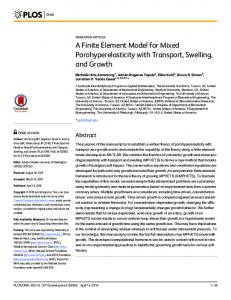
Fig. 1 Anterior, lateral, posterior, and medial views of strain rosette attachments on the tibia. Level 1 is proximal and Level 4 is at mid-diaphysis. A = anterior, P = posterior, M = medial, L = lateral.

small error in the position of load application or the assignment of material properties in the proximal region of the model would have a significant effect on the predicted strains. The aim of the current study was to create an FE model of a human cadaveric tibia and to validate it against results obtained from a comprehensive set of experiments. The authors’ intention for the model’s immediate use is to analyze artificial knee joints, so priority was given to the accuracy of the model at the proximal end. A full tibia model was created, however, in order to increase its potential applications.

2

Methods

Surface strains and displacements of a human cadaveric tibia were measured under a variety of loading conditions applied using a materials testing machine. An FE model was created based on computed tomography 共CT兲 scans. The mechanical tests were simulated using the model and the results compared to those from the experiments. 2.1 Experiments. A fresh frozen cadaveric tibia of a 60 year old Caucasian male whose cause of death was myocardial infarction, and was free of diabetes, osteoarthritis of the knee or ankle or any other bone related disease, surgery, or fracture of the tibia, was obtained 共International Institute for the Advancement of Medicine, Jessup, PA兲. A set of reference axes 共bone coordinate system兲, as described by Ruff and Hayes 关11兴, was marked on the surface of the tibia to help align the bone during experiments, to correlate the experiments with the FE model, and to help in the positioning of strain gauge rosettes. Seventeen triaxial stacked strain gauge rosettes with a grid length of 3 mm 共Mod. KFG-3-120-D17-11L3M2S, Kyowa, Tokyo, Japan兲 were glued at four different levels along the tibial surface 共Fig. 1兲. Application included complete removal of soft tissues, surface degreasing first with ethanol, then with a mixture of acetone and 2-propanol 共RMS1, HBM, Darmstadt, Germany兲, waterproofing of the bone surface with polyurethane 共PU120, HBM兲, bonding with cyanoacrylate adhesive 共CC-33A, Kyowa Electronic Instruments, Japan兲, and further protecting with two coats of polyurethane 共PU120兲 following an established procedure 关12兴. Strains were measured and recorded at 10 Hz by 031016-2 / Vol. 130, JUNE 2008

means of a 45-channel data logger 共System 6000, Vishay Measurements Group, Malvern, PA兲 interfaced with a computer, where they were stored and processed with STRAINSMART 6000 software 共Vishay Measurements Group兲. Strains were measured while the bone was subjected to a series of simplified loading scenarios 共two bending load conditions, nine axial loading conditions, and a torsional loading condition兲. All tests were performed on a biaxial testing machine 共MTS 858 MiniBionix, MTS, Minneapolis, MN兲, with the bone thawed to room temperature and kept moist, by cladding with wet swabs and periodically spraying it with water. A four-point bending jig with rollers at 62 mm intervals was used to bend the tibia in the anteroposterior plane and in the mediolateral plane with the posterior side and the lateral side in tension, respectively, following a procedure used in other studies and adopted from recommendations for testing intramedullary nails 共ASTM standard F382-86兲 关13兴. A clamp, which sat on the distal roller attached to the tibia, prevented the tibia from rotating while a 500 N load was applied. Only the strains from rosettes at Levels 3 and 4 共Fig. 1兲 were recorded during these loading conditions since the other rosettes did not experience any significant strain. In addition to strains, mid-diaphysial deflection was measured using a single-arm extensometer 共Mod. 632.06H-20, MTS, Minneapolis, MN兲. Six repetitions were performed for each bending plane, dismantling and reattaching the clamp between repetitions. For the axial loading experiments, the distal end of the tibia, to a depth of 30 mm, was potted in a steel box using bone cement, which met the ISO 5833 requirements. This box was clamped to the base of the testing machine to rigidly hold the bone in a vertical position. Vertical loads of 300 N were applied at nine different points on the tibial plateau so as to cover the regions on which the resultant contact loads were transmitted from the femur 共Fig. 2兲. It was originally intended to use ten points on the tibial plateau, but the cancellous bone under one point was damaged when loaded to 700 N, the originally planned axial load. The load was applied through a 6 mm diameter steel ball attached to a steel rod. The tibial plateau was prepared with ten small wells approximately 2 mm deep at load application points to guarantee repeatability and good contact between the ball and the bone. A set of horizontal cross rails was fitted between the rod and the loading Transactions of the ASME

Downloaded 02 May 2008 to 137.204.148.73. Redistribution subject to ASME license or copyright; see http://www.asme.org/terms/Terms_Use.cfm

Anterior LM ( not used due to damage)

Y

LA

ML MA

LC MM LL

~12 mm

Lateral

X

~12 mm

LP

Medial

MC ~8 mm

MP

~8mm

Posterior Fig. 2 Transverse view of proximal end of the tibia showing the nine points at which the 300 N axial load was applied. The first letter of each label indicates the condyle, and the second letter the location within the condyle: A = anterior, P = posterior, M = medial, L = lateral, C = central.

ram in order to ensure that the load on the bone was purely vertical. Readings from only 15 of the 17 rosettes 共all except two of the rosettes on Level 3兲 were recorded due to the maximum number of recordable channels being 45. Two dial gauges 共Mod. 2046EB-08, Mitutoyo, Japan: resolution 0.01 mm, range 10 mm兲 measured the posterior displacement and the lateral displacement at two predetermined points on the proximal bone with respect to the frame of the testing machine. Ten repetitions were carried out for each loading point. Once the axial tests had been completed on the intact cadaveric tibia, a medial tibial component of a Phase-3 Oxford Unicompartmental Knee Replacement 共Biomet, Swindon, UK兲 was implanted using the cemented 共Palacos ® R, Biomet Merck GmbH, Kerzers, Switzerland兲 procedure and the recommended surgical tools. Further axial tests were done by applying loads at five points on the component. The points were similarly positioned to those on the intact tibia. Each of the five points on the component was marked using a 1 mm diameter blind hole. The rod through which the load was applied was tapered to a point. This point was made to rest in the 1 mm hole during loading. This assured repeatability of the tests and reproducibility in the FE model. Since there was no danger of damaging the bone, a 700 N load was applied for these axial tests. Ten repetitions were performed on each loading condition. For the torsional experiment, the proximal 24 mm of the tibia were then potted in a steel box using cement, following a previously established procedure 关13兴. A system of hinges and cross rails was used again to avoid transmission of any load component other than the intended torque 共Fig. 3兲. An internal rotation torque of 20 Nm was applied while the strain readings at Levels 2, 3, and 4 were recorded 共the five rosettes on Level 1 were now either fully or partially buried in the proximal cement pot兲. Ten repetitions were carried out disconnecting the proximal pot from the loading ram between repetitions. Upon visual inspection, no physical damage caused by the experiments was observed on the bone except the local damage due to the axial loading at point LM 共Fig. 2兲. All loads were measured using a load transducer fitted under the tibia, which was able to measure the vertical load and the torsional load about the vertical axis. For all loading conditions, the maximum loads were reached with a 20 s ramp. As in previous work, the bone was allowed to creep under the peak load for a constant time of 30 s enabling reproducible measurements 关6兴. For all analysis purposes, the average of 15 readings close to the end of the 30 s load hold was Journal of Biomechanical Engineering

computed for each strain gauge. For each loading scenario, the means and standard deviations of the maximum and minimum principal strains at each rosette were calculated over all repetitions. As an indication of experimental repeatability, the overall average standard deviation and the maximum standard deviation for all rosettes under all axial loads were calculated. Similar values were calculated for the four-point bending and the torsional tests. Between load repetitions, the bone was left unstressed for a minimum of 5 min in order to relieve any residual strains. All points at which the loads were applied and the rosettes were attached, together with a large number of points distributed on the bone’s and the implant’s surface, were digitized using a digitizing arm 共MicroScribe G2, Immersion Corporation, CA兲, whose stated accuracy was 0.38 mm. The digitizing was performed so that the FE model could be transformed into the bone coordinate system, and the load application points and rosette attachment points could be located on the model.

Fig. 3 Experimental setup for torsional loading with enlarged view of proximal pot assembly. The distal pot was rigidly fixed on the load transducer „not shown…, which was fixed on the testing machine. The proximal end was twisted through the crosshead, a sliding joint, and a cross „universal… joint.

JUNE 2008, Vol. 130 / 031016-3

Downloaded 02 May 2008 to 137.204.148.73. Redistribution subject to ASME license or copyright; see http://www.asme.org/terms/Terms_Use.cfm

Table 1 Relationships used to calculate orthoropic material properties used in the FE model. CT was the CT number in Hounsfield units, ␳ was the apparent density of bone at a point, ␳c was the apparent density of corticial bone „1888 kg/ m3 derived from Refs. †17,19‡…. ␳w was the apparent density of water „1000 kg/ m3…, RD was the radiographic density at a pixel, RDc was the mean radiographic density of cortical bone „2671…, RDw was the mean radiographic density of water „1020…, RDa was the mean radiographic density of air „77…, E was Young’s modulus, and G was the shear modulus. Subscripts 1, 2, and 3 were the medial, anterior, and axial directions. Cancellous bone 共␳ ⬍ 1000 kg/ m3 关19兴兲 共corresponds to RD⬍ 1936兲 CT number in Hounsfield units Apparent density ␳ 共kg/ m3兲

Young’s Modulus E 共GPa兲

CT= 1000

共RD− RDw兲 共RDw − RDa兲

关17兴

␳ = 114+ 0.916CT 关17兴

E3 =

Cortical bone 共␳ 艌 1000 kg/ m3 关19兴兲 共corresponds to RD艌 1936兲

0.51␳1.37 关17兴 1000 E1 = 0.574E3 E2 = 0.577E3

␳c − ␳w 共RD− RDw兲 RDc − RDw Linear interpolation between two known data points 关20兴 ␳ = RDc +

E3 = −3.842+ 0.013␳ 关17兴 Derived from Ref. 关19兴

Shear Modulus G 共GPa兲

G12 = 0.195E3 G23 = 0.265E3 G31 = 0.216E3

Derived from Ref. 关19兴

Poisson’s Ratio ␯

␯12 = 0.427 ␯23 = 0.234 ␯31 = 0.405

Derived from Ref. 关19兴

2.2 Finite Element Analysis. Prior to mechanical testing, the cadaveric tibia was CT 共HiSpeed CT/i, GE Medical Systems兲 scanned in the transverse direction while submerged in water to reduce beam-hardening artifacts. The scans were taken at 1 mm intervals for the most proximal 80 mm and the most distal 60 mm of the tibia, and at 3 mm intervals along the diaphysis; the pixel size was 0.23⫻ 0.23 mm2. The scanner parameters were 120 KVP and an X-ray tube current of 160 mA. The CT images were segmented and used to create a 3D geometric model of the tibial surface 共SLICEOMATIC, Version 4.2 Rev-9b, TomoVision, Virtual Magic Inc., Montreal, Canada兲. The surface geometry was transformed into the bone based coordinate system used during mechanical testing using an iterative closest point 共ICP兲 algorithm 关14兴. Digitized points on the bone at which rosettes were attached and at which displacements were measured were then located on the surface geometry. Five FE meshes of ten-node tetrahedral elements with varying refinement 共12,993–113,759 nodes兲 were created using PATRAN 共MSC.Patran, 2004 r2, MSC.Software Corporation, Santa Ana, CA兲 in order to check for convergence of principal strains, deflections, and strain energy. A mesh consisting of 75,583 nodes was found to have sufficiently converged 共giving a strain energy gradient of 3.60⫻ 10−06% per unit increase in degree of freedom 关15兴兲 and this mesh was used for further analysis. Assignment of material properties was automated using a custom written MATLAB routine 共MATLAB Version 7.0, The Maths Works, Natick, MA兲, which calculated the material properties on an element by element basis. The sampling points were spaced at 0.23 mm, 0.23 mm, and 0.23/ 8 mm in the x, y, and z directions, respectively. A special algorithm was used to make sure that all sampling points used to calculate material properties of an element were within the bone 关16兴. To reduce errors caused due to the partial volume effects, a more refined mesh was used nearer the bone’s surface. Each element was assigned one of the 600 orthotropic material properties calculated from CT data. A separate study performed using the same mesh revealed that 600 ma031016-4 / Vol. 130, JUNE 2008

terial properties were sufficient to accurately model the tibia 关16兴. Relationships established by Rho et al. 关17–19兴 were used to derive orthotropic material properties from CT intensities 共Table 1兲. The anisotropy was assumed to be the same throughout the whole bone. That is, the Young’s moduli of an element in the anteroposterior and mediolateral directions were assumed to be constant multiples of Young’s modulus in the axial direction. These two constants 共0.577 and 0.574, Table 1兲 were calculated by finding the mean of the ratios between axial Young’s modulus and anteroposterior and mediolateral Young’s moduli at 12 sampling points in cortical bone used by Rho et al. 共Fig. 3 and Table 2 关19兴兲. The same constants were assumed for cancellous bone. The range of Young’s moduli in the axial direction varied from approximately

Table 2 Largest values for experimental principal strains and standard deviations for axial, four-point bending, and torsional loading Axial loading Intact Implanted Bending Torsion Minimum principal strain

Maximum principal strain

Largest value −569 共microstrain兲 Largest standard 24.6 deviation 共STD兲 共microstrain兲 CV corresponding to 5.9 largest STD% Largest value 共microstrain兲 Largest standard deviation 共STD兲 共microstrain兲 CV corresponding to largest STD%

−1366

−660

−1029

29.8

43.0

10.0

2.2

26.1

1.7

426

807

654

1020

19.7

14.7

58.1

8.7

5.9

2.5

25.8

0.9

Transactions of the ASME

Downloaded 02 May 2008 to 137.204.148.73. Redistribution subject to ASME license or copyright; see http://www.asme.org/terms/Terms_Use.cfm

Fig. 4 The distribution of axial Young’s modulus along the tibia. Each point represents an element

14 MPa to 22,100 MPa 共Fig. 4兲. The mechanical tests were simulated using the FE model, assuming nonlinearity due to large displacements 共MSC.MARC, 2003, MSC.Software Corporation, Santa Ana, CA兲. The displacement at each point at which it was measured, and the maximum and minimum principal strains at each rosette attachment site in the plane of the rosette were calculated. The axial loading condition was simulated by fixing the surface nodes up to 30 mm from the distal end in all directions. A vertically downward point load of 300 N 共or 700 N for the implanted tibia兲 was applied at the node, which represented the load application point. This was repeated for all the loading points. The implant, cement, and bone were assumed to be rigidly bonded. Four-point bending was simulated by fixing the nodes nearest the bottom rollers in the appropriate directions 共Fig. 5兲. The two top rollers were simulated with two equal point displacements, which gave a total reaction load of 500 N. The correct displacement for the points was found by an iterative procedure. The torsional loading condition was simulated as follows: Similar to the axial loading case, the surface nodes at the distal end were fixed in all directions. The torque was simulated by applying two parallel and opposite point loads at the periphery of the proximal tibial plateau to produce a 20 Nm torque. Different point and load combinations 共which all gave a 20 Nm torque兲 were tried and they each gave similar strain results. The applied torque with

Nodes fixed in y direction to prevent tibia rotating

z x

the smallest loads and the greatest distance between them 共259.7 N and 77.0 mm兲 was used to minimize the local effects at loading points. 2.3 Experiment and FE Model Comparisons. For each axial load case, the rosettes within a distance of 31 mm from the loading point were not considered in the analysis. This criterion meant that for the 14 axial loading conditions, two rosettes were ignored for 2 of the loading conditions and one rosette each was ignored for 11 of the loading conditions. This exclusion was based on Saint-Venant’s principle and was done to minimize the error caused by representing the experimental loads by point loads in the FE model. The distance of 31 mm was selected by observing the accuracy of the collective results while progressively excluding the results of the nearest rosette. Once the results of the rosettes within 31 mm of the load application points were rejected, further exclusion of rosettes had little influence on the overall results. Regression lines were found for plots of strains predicted by the FE model versus experimentally measured strains for each loading condition separately, as well as all of the axial loading conditions combined. As another indicator of accuracy of the FE model, the root mean square error 共RMSE兲 was calculated. The RMSEs for axial, bending, and torsional loads were expressed as percentages of the peak of the absolute values of principal strains measured under each loading condition. This value was termed

Equal displacement in -x direction giving a total of 500 N (top rollers)

Nodes fixed in x, y, and z directions to prevent rigid body motion (distal bottom roller)

Nodes fixed in x direction (proximal bottom roller)

Fig. 5 The intact cadaveric tibia FE model together with the boundary conditions used to simulate four-point bending in the mediolateral direction

Journal of Biomechanical Engineering

JUNE 2008, Vol. 130 / 031016-5

Downloaded 02 May 2008 to 137.204.148.73. Redistribution subject to ASME license or copyright; see http://www.asme.org/terms/Terms_Use.cfm

Fig. 6 FE model principal strains plotted against experimental principal strains for all nine axial load cases combined, along with the best fit regression line for the intact cadaveric tibia

RMSE% and has been used by others 关1,5,6兴 to express the accuracy of their models. The errors in deflections under axial loading were calculated as a percentage of the largest deflection measured under all axial loads. All error calculations were done in comparison to the measured values.

3

Results

3.1 Experiments. The experimental results were highly repeatable 共Table 2兲. For example, the largest standard deviation in principal strains between repeated measurements for axial loading was 29.8 microstrain, which corresponded to a coefficient of variation 共CoV兲 of 2.2%. Torsional loading gave the most repeatable results where the largest CoV in principal strains for any strain rosette was 2.7%. The mid-diaphyseal deflections during four-point bending were 0.27 mm in anteroposterior bending and 0.29 mm in mediolateral bending. The CoVs for both these values were less than 8%. The anteroposterior and mediolateral bending stiffnesses were 1852 N / mm and 1724 N / mm, respectively. During axial loading of the intact tibia to 300 N, the mean experimental deflections varied between 0.01 mm and 1.29 mm in the anteroposterior plane, and between 0.59 mm and 1.94 mm in the mediolateral plane. For loads applied at points MM, ML, and LA 共Fig. 2兲, the deflections in the anteroposterior plane were small 共⬍0.1 mm兲 and varied in direction between repetitions. During axial loading of the implanted tibia to 700 N, the mean experimental deflections varied between 0.11 mm and 3.63 mm in the anteroposterior plane, and between 2.09 mm and 4.70 mm in the mediolateral plane. 3.2 Experiment and FE Model Comparison. For the intact tibia, the regression line of principal strains for all axial load cases combined had a slope of 1.15, an intercept of 5.46 micro strain, an R2 of 0.98, and a RMSE% of 6.0% 共Fig. 6, Table 3兲. Considering the individual axial load cases, the least accurate results were given for the load applied at the point ML. The results for this load application point gave the largest RMSE 共16%兲, the most 031016-6 / Vol. 130, JUNE 2008

erroneous slope 共1.31兲, and smallest value for R2 共0.96兲 共Table 3兲. For the implanted tibia, the regression line of principal strains for all axial load cases combined had a slope of 1.25, an intercept of 12.3 microstrain, an R2 of 0.97, and a RMSE% of 8.8% 共Fig. 7, Table 3兲. For the implanted tibia, too, the least accurate results were given for the load applied at the point ML. The results for this load application point gave the largest RMSE 共18%兲, the most erroneous slope 共1.35兲, and smallest value for R2 共0.95兲 共Table 3兲. For four-point bending, the combined regression line had a slope of 1.06, an intercept of −1.9 microstrain, and an R2 value of 0.96. The RMSE% was 9.0%. The most accurate results were obtained for the torsional loading condition where the slope, intercept, and R2 were 1.02, −11.73 microstrain, and 0.99, respectively. The RMSE% for torsion was 6.3%. The intercepts of the regression lines under all loading conditions were small in comparison to the largest measured strain under each loading condition 共⬍2 % 兲. Under axial loading of the intact tibia, all errors in deflections were less than 20% of the largest measured deflection, which was 1.94 mm 共Table 4兲. The largest error occurred in the predicted deflection in the anteroposterior plane for the condition where the load was applied at MM. For axial loads applied at MM, ML, and LA, where the deflections in the anteroposterior plane were 0.03 mm posterior, 0.01 mm anterior, and 0.09 mm anterior, respectively, the predicted deflections were in the opposite direction to those measured but still very small in magnitude. Under axial loading of the implanted tibia, all but one error in deflection was less than 17.5% of the largest measured deflection, which was 4.70 mm 共Table 4兲. Under four-point bending, the model was stiffer than the tibia and predicted mid-diaphyseal deflections of 0.22 mm in anteroposterior bending and 0.25 mm in mediolateral bending. These values were 17% and 12% less than the respective measured values. Transactions of the ASME

Downloaded 02 May 2008 to 137.204.148.73. Redistribution subject to ASME license or copyright; see http://www.asme.org/terms/Terms_Use.cfm

Table 3 The slope, intercept, R2, and the RMSE for the nine axial loading conditions on intact tibia, the four-point bending in two directions, the torsional loading condition, and the five axial loading conditions on the implanted tibia. RMSE is given as a percentage of the largest measured strain under each loading condition. Slope

Intercept 共micro strain兲

R2

RMSE 共%兲

Axial load at MC Axial load at MM Axial load at MP Axial load at ML Axial load at MA Axial load at LC Axial load at LL Axial load at LP Axial load at LA All axial loading results combined Four-point bending in anteroposterior direction Four-point bending in mediolateral direction Four-point bending results combined

1.153 1.159 1.147 1.307 1.145 1.148 1.102 1.145 1.170 1.146 1.133

3.4 5.2 4.9 4.8 4.8 7.0 7.9 11.3 2.9 5.5 −3.4

0.973 0.974 0.972 0.961 0.988 0.988 0.986 0.986 0.985 0.980 0.967

10.2 7.4 11.7 16.0 8.0 8.6 7.5 9.3 9.5 6.0 11.2

1.008

−1.4

0.962

9.0

1.059

−1.9

0.961

9.0

Axial load at MC Axial load at MM Axial load at MP Axial load at ML Axial load at MA All axial loading results combined Torsional loading condition

1.214 1.250 1.255 1.352 1.227 1.246 1.018

8.0 14.3 21.7 9.9 11.0 12.3 −11.7

0.971 0.967 0.953 0.953 0.981 0.966 0.994

12.2 11.6 9.1 18.4 12.1 8.8 6.3

Loading condition Intact tibia

Implanted tibia

4

Discussion

The FE models of an intact and implanted human cadaveric tibia were created and validated against a comprehensive set of experiments in which applied forces, surface strains, and displacements were measured under axial, bending, and torsional loads. The experimental results for bending stiffnesses in the anteropos-

terior and mediolateral directions were well within the wide range of values reported elsewhere. The reported range for bending stiffness in the anteroposterior and in the mediolateral directions were 854– 2787 N / mm and 637– 2547 N / mm, respectively 关13兴. The FE models were able to predict the mechanical behavior of the human cadaveric tibia to acceptable accuracy under axial 共for

Fig. 7 FE model principal strains plotted against experimental principal strains for all five axial load cases combined, along with the best fit regression line for the implanted cadaveric tibia

Journal of Biomechanical Engineering

JUNE 2008, Vol. 130 / 031016-7

Downloaded 02 May 2008 to 137.204.148.73. Redistribution subject to ASME license or copyright; see http://www.asme.org/terms/Terms_Use.cfm

Table 4 The errors in predicted deflections in lateral and posterior directions for nine axial load cases for the intact tibia and the implanted tibia. Errors are given as a percentage of the maximum measured deflection under axial loading „1.94 mm for the intact tibia and 4.70 mm for the implanted tibia…. The values marked with “ *” are instances where the average measured deflection was in the opposite direction to the predicted deflection. The negative values indicate that the predicted result was smaller than the measured value.

Intact tibia Implanted tibia

Posterior Lateral Posterior Lateral

MC

MM

MP

ML

MA

LC

LL

LP

LA

6.7% 1.4% 8.3% 4.5%

* 19.8%

−1.5% 3.4% −17.2% 12.3%

* 4.4%

4.5% 3.1% −1.1% 10.2%

16.3% 2.0%

17.2% −9.5%

12.8% 0.4%

* 6.1%

2.1% 24.7% 10.9%

16.6% 12.8% 15.5%

the intact tibia R2 = 0.98, RMSE% = 6.0 and for the implanted tibia R2 = 0.97, RMSE% = 8.8兲, bending 共R2 = 0.96, RMSE% = 9.0兲, and torsional 共R2 = 0.99, RMSE% = 6.3兲 loads 共Table 3兲. Since there are no published results for a similar study on a human cadaveric tibia, comparisons were made between the relative accuracies of this study with the accuracy of validated FE models of the composite tibia and cadaveric and composite femurs. All parameters 共slope and R2 of regression line and RMSE%兲 were within the range of those published 共Table 5兲. The errors in deflections under axial loading are within those reported for a validated model of a composite tibia 关3兴, where the errors range from 0.5% to 27%. None of the other validation studies has reported the errors in deflections. There could be many reasons for the FE model to appear less rigid than the cadaveric tibia under axial loading. One reason may be that material properties assigned to the model were lower than the actual values. Another reason could be that the cross rails used to eliminate the horizontal loads were not smooth enough and applied a frictional force. This force would be opposite to the direction in which the bone was bending, and therefore would reduce the amount the bone bent causing it to appear more rigid. This, however, is an error in the boundary conditions and therefore is not inherent to the model and will not affect the accuracy of results under other boundary conditions. For axial loading, the worst errors were given for the case where the load was applied at ML. The slope, the R2 value, and the RMSE% all indicated that the predictions by the model were least accurate for this loading condition. ML is also the closest of the 14 load application points to the midsagittal plane of the tibia. In general, the model’s accuracy increased 共with decreasing slope of the regression line兲 when the loading point was further away from the midsagittal plane 共Table 3兲. This again could be due to the presence of a frictional force in the cross rails, as explained above. Another reason could be that a small error in positioning the load application point on the model would have a greater influence if the distance from the point to the neutral plane was smaller. The deflections of the proximal tibia under axial loading for the intact tibia compared well to the model 共all errors except for 5 were less than 10%兲. For the implanted tibia, the errors were

8.8%

larger. Only in four cases were the predicted deflections smaller than those measured. This is in agreement with the strain comparison, which suggested that the model was less rigid than the bone or that the applied boundary conditions were inaccurate. In some cases 共loads applied at MM, ML, and LA for the intact tibia兲, the predicted deflections in the anteroposterior plane were in the opposite direction to those measured. These measured deflections were very small and were in different directions between repetitions, indicating that the loading points were on or very close to the neutral plane of the bone parallel to the mediolateral plane. A small error in the position of load application in the model will change the direction of the predicted deflection. The minimum R2 value for combined loading conditions was given for four-point bending 共R2 = 0.96兲. However, this R2 value, the slope 共1.06兲, and the RMSE% 共9.0%兲 are within accuracy levels published by others for validation studies done using femurs. The errors in predicted mid-diaphyseal deflections were rather large 共17% and 12%兲. Perhaps this is due to a change in the point at which mid-diaphyseal deflection was measured as the cadaveric tibia was twisted during loading. For the model, twisting did not change the point at which the deflection was calculated because the deflection was calculated at a particular node.

5

Conclusion

This study compared the principal strains and displacements at selected points, measured by experiments on a human cadaveric tibia, to those predicted by an FE model based on the same bone. Only surface strains were compared as the measurement of internal strains is experimentally difficult; however, it is reasonable to assume that the internal strains will be accurate if the external strains and the material property assignment were accurate. The model produced by the current study provides a tool for simulating mechanical test conditions on a human tibia. This has considerable value in reducing the costs of physical testing by pre-selecting the most appropriate test conditions or most favorable prosthetic designs for final mechanical testing. It can also be used to gain insight into the results of physical testing, by allowing the prediction of those variables difficult or impossible to measure directly. The model is now being used to analyze the

Table 5 Comparison of accuracy of model for combined results for axial, combined results for bending, and results for torsional loading conditions with accuracy levels of other published studies on cadaveric and composite tibia and femur surface strains

Slope of regression line R2 RMSE%

This study

Composite tibia model 关3兴

Cadaveric femur model 关4兴

Cadaveric femur model 关6兴

Composite femur model 关1兴

Composite femur model 关5兴

1.018–1.246

0.999–1.280

0.897

1.010

0.92–1.05

0.85–0.89

0.961–0.994 6.0–9.0

0.947–0.964 5.0–21.4

0.835 –

0.910 8.6

0.977–0.992 5.6–10.0

0.98 9.5–11.3

031016-8 / Vol. 130, JUNE 2008

Transactions of the ASME

Downloaded 02 May 2008 to 137.204.148.73. Redistribution subject to ASME license or copyright; see http://www.asme.org/terms/Terms_Use.cfm

bone implant interface under the tibial component of the unicompartmental knee replacement in order to better understand the cause for radiolucency.

关9兴

Acknowledgment

关10兴

H. G. held a Felix Scholarship at the University of Oxford. He was awarded a Charterhouse European Bursary to travel to Bologna, Italy, where all experiments were performed. The authors wish to thank Dr. Marco Viceconti of the Istituti Ortopedici Rizzoli, Bologna, for providing the CT scans of the tibia.

关11兴 关12兴

References 关1兴 Stolk, J., Verdonschot, N., Cristofolini, L., Toni, A., and Huiskes, R., 2002, “Finite Element and Experimental Models of Cemented Hip Joint Reconstructions Can Produce Similar Bone and Cement Strains in Pre-Clinical Tests,” J. Biomech., 35共4兲, pp. 499–510. 关2兴 Fagan, M., 1997, Finite Element Analysis: Theory and Practice, Longman, Singapore. 关3兴 Gray, H. A., Zavatsky, A. B., Taddei, F., Cristofolini, L., and Gill, H. S., 2007, “Experimental Validation of a Finite Element Model of a Composite Tibia,” Proc. Inst. Mech. Eng., Part H: J. Eng. Med., 221, pp. 315–324. 关4兴 Lengsfeld, M., Schmitt, J., Alter, P., Kaminsky, J., and Leppek, R., 1998, “Comparison of Geometry-Based and CT Voxel-Based Finite Element Modelling and Experimental Validation,” Med. Eng. Phys., 20共7兲, pp. 515–522. 关5兴 Waide, V., Cristofolini, L., Stolk, J., Verdonschot, N., Boogaard, G. J., and Toni, A., 2004, “Modelling the Fibrous Tissue Layer in Cemented Hip Replacements: Experimental and Finite Element Methods,” J. Biomech., 37共1兲, pp. 13–26. 关6兴 Taddei, F., Cristofolini, L., Martelli, S., Gill, H. S., and Viceconti, M., 2006, “Subject-Specific Finite Element Models of Long Bones: An In Vitro Evaluation of the Overall Accuracy,” J. Biomech., 39共13兲, pp. 2457–2467. 关7兴 Duda, G. N., Mandruzzato, F., Heller, M., Goldhahn, J., Moser, R., Hehli, M., Claes, L., and Haas, N. P., 2001, “Mechanical Boundary Conditions of Fracture Healing: Borderline Indications in the Treatment of Unreamed Tibial Nailing,” J. Biomech., 34共5兲, pp. 639–650. 关8兴 Duda, G. N., Mandruzzato, F., Heller, M., Kassi, J. P., Khodadadyan, C., and

Journal of Biomechanical Engineering

关13兴 关14兴 关15兴

关16兴 关17兴 关18兴 关19兴 关20兴

Haas, N. P., 2002, “Mechanical Conditions in the Internal Stabilization of Proximal Tibial Defects,” Clin. Biomech. 共Bristol, Avon兲, 17共1兲, pp. 64–72. Perillo-Marcone, A., Barrett, D. S., and Taylor, M., 2000, “The Importance of Tibial Alignment: Finite Element Analysis of Tibial Malalignment,” J. Arthroplasty, 15共8兲, pp. 1020–1027. Perillo-Marcone, A., Alonso-Vazquez, A., and Taylor, M., 2003, “Assessment of the Effect of Mesh Density on the Material Property Discretisation Within QCT Based FE Models: A Practical Example Using the Implanted Proximal Tibia,” Comput. Methods Biomech. Biomed. Eng., 6共1兲, pp. 17–26. Ruff, C. B., and Hayes, W. C., 1983, “Cross-Sectional Geometry of Pecos Pueblo Femora and Tibiae—A Biomechanical Investigation: I. Method and General Patterns of Variation,” Am. J. Phys. Anthropol., 60共3兲, pp. 359–381. Viceconti, M., Toni, A., and Giunti, A., 1992, “Strain Gauge Analysis of Hard Tissues: Factors Influencing Measurements,” Experimental Mechanics. Technology Transfer Between High Tech Engineering and Biomechanics, E. G Little, ed., Elsevier Science, Amsterdam, pp. 177–184. Cristofolini, L., and Viceconti, M., 2000, “Mechanical Validation of Whole Bone Composite Tibia Models,” J. Biomech., 33共3兲, pp. 279–288. Estépar, R. S. J., Brun, A., and Westin, C.-F., 2004, “Robust Generalized Total Least Squares Iterative Closest Point Registration,” Medical Image Computing and Computer-Assisted Intervention—MICCAI 2004, pp. 234–241. Polgar, K., Viceconti, M., O’Connor, J. J., 2001, “A Comparison Between Automatically Generated Linear and Parabolic Tetrahedra When Used to Mesh a Human Femur,” Proc. Inst. Mech. Eng., Part H: J. Eng. Med., 215共1兲, pp. 85–94. Gray, H. A., 2007, “Finite Element Analysis of the Human Tibia,” Ph.D. thesis, University of Oxford, Oxford. Rho, J. Y., Hobatho, M. C., and Ashman, R. B., 1995, “Relations of Mechanical Properties to Density and CT Numbers in Human Bone,” Med. Eng. Phys., 17共5兲, pp. 347–355. Rho, J. Y., Ashman, R. B., and Turner, C. H., 1993, “Young’s Modulus of Trabecular and Cortical Bone Material: Ultrasonic and Microtensile Measurements,” J. Biomech., 26共2兲, pp. 111–119. Rho, J. Y., 1996, “An Ultrasonic Method for Measuring the Elastic Properties of Human Tibial Cortical and Cancellous Bone,” Ultrasonics, 34共8兲, pp. 777– 783. Zannoni, C., Mantovani, R., and Viceconti, M., 1998, “Material Properties Assignment to Finite Element Models of Bone Structures: A New Method,” Med. Eng. Phys., 20共10兲, pp. 735–740.

JUNE 2008, Vol. 130 / 031016-9

Downloaded 02 May 2008 to 137.204.148.73. Redistribution subject to ASME license or copyright; see http://www.asme.org/terms/Terms_Use.cfm