Experiments with EOF-Based Perturbation Methods ... - AMS Journals

1438

MONTHLY WEATHER REVIEW

VOLUME 137

Experiments with EOF-Based Perturbation Methods and Their Impact on the CPTEC/INPE Ensemble Prediction System ANTOˆNIO MARCOS MENDONCx A AND JOSE´ PAULO BONATTI Center for Weather Prediction and Climate Studies (CPTEC), National Institute for Space Research (INPE), Cachoeira Paulista, Saõ Paulo, Brazil (Manuscript received 4 March 2008, in final form 28 August 2008) ABSTRACT The impact of modifications of the perturbation method based on empirical orthogonal functions (EOFs) used operationally upon the ensemble prediction system (EPS) at the Center for Weather Prediction and Climate Studies/National Institute for Space Research (CPTEC/INPE) is evaluated. The main changes proposed in this study are to apply the EOF method to perturb the midlatitudes, apply additional perturbations to the surface pressure (P) and specific humidity (Q) fields, and compute regional perturbations over South America. The impact of these modifications in the characteristics of the initial perturbations and in the quality of the EPS forecasts is investigated. The EPS forecasts are evaluated through average statistical scores over the period 15 December 2004–15 February 2005. The statistical scores used in the evaluation are pattern anomaly correlation, root-mean-square error, ensemble spread, Brier skill score, and perturbation versus error correlation analysis (PECA). Results indicate that with the inclusion of perturbations on P and Q, EOF-based perturbations acquire a more baroclinic structure. It is also observed that the simultaneous application of additional perturbations both in the extratropics and to the P and Q fields improves the performance of CPTEC EPS and enhances the quality of forecast perturbations. Moreover, regional EOFbased perturbations computed over South America have positive impact on the ensemble forecasts over the target region.

1. Introduction Atmospheric forecasts with high skill are an objective and at the same time a challenge to numerical weather prediction. To increase the quality of the numerical weather forecasts, two main factors must be taken into account: the representation of physical and dynamical processes in the atmosphere by numerical models, and an initial condition that realistically reproduces the atmospheric state at the beginning of the model integration. The fast development of computational technology over the last few decades has provided conditions for a better representation of the physical and dynamical atmospheric processes by numerical models. At the same time, the advent of the meteorological satellite information has significantly increased the quantity of data that, in addition to demanding improvements in the

Corresponding author address: Antoˆnio Mendoncxa, CPTEC/ INPE, Rod. Presidente Dutra, Km 40, Cachoeira Paulista, CEP 12630-000, Saõ Paulo, Brazil. E-mail: [email protected] DOI: 10.1175/2008MWR2581.1 Ó 2009 American Meteorological Society

methods of data assimilation (Hamill 2002; Kalnay et al. 2002; Rabier et al. 2000) has contributed to producing high-quality analyses. However, despite the advances in representing atmospheric processes by numerical models and the production of accurate analyses, numerical forecasts diverge from observed atmospheric evolution after some days of model integration. The sources of numerical weather forecast errors are mainly the two previously described factors: deficiencies of the models in representing dynamical and physical processes of the real atmosphere, or the external error; and uncertainties in the state of the atmosphere at the initial time, or the internal error (Reynolds et al. 1994). The model uncertainties were considered in the development of ensemble forecasting systems that run the model a number of times with different parameterization schemes to create a set of perturbed forecasts (Krishnamurti et al. 2000; Houtekamer et al. 1996). The model uncertainties were also treated following a method described by Buizza et al. (1999). In their scheme, the random model errors due to the physical parameterization processes are simulated by including

APRIL 2009

M E N D O N Cx A A N D B O N A T T I

stochastic perturbations in the parameterized diabatic tendency for any component of the state vector. The importance of the initial-state uncertainties in forecast errors is explained by chaos theory which, in a simplified form, is related to the sensitivity that some nonlinear deterministic dynamic systems exhibit with respect to initial and boundary conditions as they evolve in time (Lorenz 1963, 1965, 1969). The atmosphere is an example of a chaotic system (i.e., slightly different initial conditions may lead to significantly different final solutions). Thus, even in a perfect model scenario, since the atmospheric state is not completely represented by the analyses, the unavoidable errors will grow as the model evolves with time, degrading the quality of forecast until it eventually lacks any useful skill. Some ensemble weather prediction systems do not take into account the uncertainties in numerical models and consider only the uncertainties in the initial conditions. In these systems, one of the most important characteristics is the strategy used to generate the perturbed analysis. Under the perfect-model hypothesis, they try to estimate perturbations that have potential to grow in time and can produce a set of forecasts that are diverse enough to give an impression of the likely range of future atmospheric states (Buizza et al. 1999). The National Centers for Environmental Prediction (NCEP) and the European Centre for Medium-Range Weather Forecasts (ECMWF) in 1992 were the centers that pioneered in the implementation of operational ensemble weather forecasting. They used the methods of breeding of growing modes (Toth and Kalnay 1993) and singular vectors (Molteni et al. 1996) to generate perturbed initial conditions. Later, other methods for generating perturbed analysis and ensemble forecasting were developed, such as the perturbed-observation approach (Houtekamer et al. 1996) and more recently, perturbation methods based on ensemble Kalman filters (Wei et al. 2006; Houtekamer et al. 2005; Ott et al. 2004; Wang and Bishop 2003; Bishop et al. 2001). Zhang and Krishnamurti (1999, hereafter ZK99) developed a procedure for generating initial ensemble perturbations based on principal component analysis called (empirical orthogonal function) EOF-based perturbations (or, the EOF method), in order to produce hurricane ensemble forecasts. In this method, those eigenvectors whose EOF coefficients increase rapidly with time are selected to generate perturbed analyses. Coutinho (1999) performed adaptations to the EOF method in order to produce perturbed initial conditions with the atmospheric general circulation model (AGCM) of the Center for Weather Prediction and Climate Studies/National Institute for Space Research (CPTEC/INPE). The ensemble forecasts initialized with

1439

the EOF method presented better results when compared with ensemble predictions based on random initial perturbations. Moreover, the EOF ensemble mean forecasts presented better performance than the control forecasts. In October 2001, the CPTEC/INPE started to produce operational ensemble weather forecasts using the approach described in Coutinho (1999). In Farina et al. (2005) the EOF method together with the CPTEC AGCM was also used to generate perturbed surface wind stress in order to force an ocean wave model and produce ocean wave ensemble predictions. Mendoncxa and Bonatti (2006) evaluated the CPTEC/ INPE ensemble prediction system (EPS) using statistical scores [i.e., anomaly correlation, root-mean-square error (rmse), standard deviation spread] and showed that, at least for 500-hPa geopotential height, the CPTEC/ INPE ensemble forecasts are underdispersive (i.e., the ensemble spread is smaller than the rmse of the ensemble mean forecasts). In an attempt to reduce this deficiency it was suggested that modifications be made in the region used to compute the initial perturbations. In the operational version, the perturbations were computed in a latitude belt between 458S and 308N for temperature and wind fields. They found that the application of the EOF method to calculate additional extratropical perturbations enhances the performance of CPTEC EPS, mainly for 24-h and 48-h forecast lead times. The influence of extratropical systems upon tropical region dynamics and vice versa was studied by Palmer (1988). Connections between anomalies in tropical atmospheric systems and the observed variability in determined extratropical regions at several time scales have been described in work by Mo and Higgins (1998), Simmons (1982), Hoskins and Karoly (1981), and others. On the other hand, the propagation of transient systems from the midlatitudes toward the tropics may be a source of energy for tropical systems. Liebmann and Hartmann (1984) concluded that on time scales of 5 to 10 days, midlatitude systems exert strong influence over the tropical atmosphere. Thus, the perturbation growth in the midlatitudes may influence the quality of the forecasts in the tropics through tropical–extratropical atmospheric interaction. Reynolds et al. (1994) found that the random error growth in the NCEP AGCM over the extratropics due to model dynamical instability is much greater than over the tropics. As a consequence, Zhang (1997) suggested that it would be better to generate perturbations over the midlatitudes and tropics separately. In view of such evidence, in this paper we investigate the influence that midlatitude EOF-based perturbations have on the quality of the CPTEC/INPE ensemble forecasts in both global and local scales, especially over South America. Moreover, we evaluate the impact of

1440


applying perturbations to the surface pressure and specific humidity, which are prognostic fields of the model but are not perturbed in the operational version of the CPTEC EPS. For evaluation, a number of experiments are carried out, in which the EOF method configuration (i.e., the region used to compute the unstable modes and perturbed fields) is modified. Each experiment is evaluated according to the structure of the initial perturbations and using average statistical scores for two months (15 December 2004–15 February 2005). Our motivation for performing this investigation is to attempt to improve the quality of the CPTEC/ INPE ensemble forecasts and demonstrate the current status of our ensemble prediction system. Brief descriptions of the dataset, the methodology used to configure the experiments, and the statistical scores computed to evaluate the results are presented in section 2. The results are discussed in section 3 and conclusions are presented in section 4.

2. Data and methodology a. Initial conditions, climatology, and period of evaluation The control initial conditions (without perturbations) used in this study are the 1200 UTC daily spectral analyses obtained from NCEP by CPTEC/INPE to produce operational ensemble weather forecasts. The horizontal spectral truncation used here is T126 (i.e., triangular truncation at zonal wavenumber 126). To avoid aliasing in the solution of nonlinear terms of model equations it is necessary to use approximately a number of points in the zonal direction equivalent to 3 times the shortest wavenumber considered, which corresponds to approximately a 0.948 latitude 3 longitude resolution in grid space. In the vertical, the atmosphere is divided into 28 sigma layers (L28). For evaluations, these initial conditions are considered as the best estimate of the real atmospheric state. For each CPTEC EPS simulation, seven EOF-based perturbations are generated and added (subtracted) to (from) the control analysis, creating a set of 14 perturbed initial conditions. Each ensemble member represents an integration of the CPTEC AGCM up to 10days lead time from a perturbed initial condition or from the control analysis. The result obtained from each EPS simulation is an ensemble of 15 members for each forecast range. The period considered for the evaluation of the experiments by use of statistical scores is from 15 December 2004 to 15 February 2005 (i.e., the Southern Hemisphere summer). In South America, climatology indicates intense convective activity over the northern

VOLUME 137

and central parts of the continent during this period. The intertropical convergence zone (ITCZ), the South Atlantic convergence zone (SACZ), the subtropical jet stream, the Bolivian high, and the northeastern Brazilian trough are the most significant synoptic-scale systems that influence the weather conditions in this region during the summer season. This period was chosen because of the relatively low predictability that numerical models exhibit over South America around this time of year, as a result of the strong role that physical processes, especially deep convection, play in the forecasts over this region. We are particularly interested in the impact of the modifications to the initial perturbations proposed in each experiment upon the quality of the ensemble forecast, especially over South America; thus, these weather forecasts have particular relevance for economic and social activities during this period. The NCEP reanalysis 2 climatology (Kanamitsu et al. 2002) is used to calculate analysis and ensemble forecast anomalies and climatological standard deviation of the 500-hPa geopotential height and of the 850-hPa horizontal wind fields.

b. CPTEC/INPE atmospheric general circulation model The model used in this study is the CPTEC AGCM at the same resolution as the analyses (T126L28). Briefly, the CPTEC AGCM is based on the spectral solution of the primitive dynamic equations in the form of divergence and vorticity, virtual temperature, specific humidity, and the logarithm of the surface pressure, and includes subgrid processes through parameterizations. Details of the model can be obtained in Kinter et al. (1997). The main physical processes included in the CPTEC AGCM are d d d d

d d

d

d

Kuo-type deep convection, shallow convection, large-scale condensation, Simplified Simple Biosphere land surface scheme (SSiB), bulk aerodynamics scheme over oceans, planetary boundary layer based on the Mellor– Yamada closure scheme, radiative fluxes (shortwave and longwave) based on a band model, and interaction of radiation with clouds.

c. The CPTEC/INPE operational EOF-based perturbation method The procedure employed to generate the perturbed atmospheric initial conditions is based on the method developed by ZK99, originally proposed for hurricane

APRIL 2009


forecasting using the Florida State University (FSU) AGCM. This method, called EOF-based perturbations, was developed because of the fact that during the first few days (around 1.5 days) of model integration, perturbations grow linearly. The procedure used at CPTEC/INPE for producing perturbed analyses can be outlined in the following steps: 1) The n random small perturbations (currently n 5 7) are added to the temperature and horizontal wind components fields of the control analysis. These perturbations are normally distributed with mean zero and standard deviation comparable to that of the 3-h forecast error (3 m s21 for the wind field and 0.6 K for the temperature field). 2) The resulting n randomly perturbed analyses and the control analysis are used to integrate the model for 36 h, with results saved every 3 h. No horizontal or vertical smoothing or balance is imposed for the random initial perturbations; however, the 6 first hours of model integration is discarded in order to allow a self-adjustment of the model to the perturbed initial conditions and consequently develop more balanced forecast perturbations. 3) The n time series of the difference field forecasts are constructed by subtracting the control forecast from the perturbed forecasts at each time increment of 3 h. 4) An EOF analysis is performed for each n time series on a domain of interest to determine the eigenvectors whose EOF coefficients increase rapidly with time. These eigenvectors are considered as the EOF perturbations. 5) These perturbations are rescaled in order to make their standard deviation of the same order as the initial perturbations. 6) Adding (subtracting) these rescaled perturbations to (from) the control analysis produces an ensemble of 2n initial perturbed states. Finding the EOF perturbations cited in item 4) consists of obtaining the directions that explain the maximum amount of variance in which the randomly perturbed forecasts diverge from the control forecast in a period of time of approximately linear growth. The EOF analysis is useful for this purpose. In this case, it is based on the solution of an eigenvalue problem of the covariance matrix obtained from the difference time series, described in item 3). Taking into account the N points over a specified domain, an M 3 N dataset matrix X of these difference time series is constructed, where M is the number of model outputs during the period from 6 to 36 h with interval of 3 h (M 5 11). The N 3 N

1441

covariance matrix is defined as C 5 (1/M)XTX, where the superscript T denotes the transpose matrix. Here C is a symmetric matrix. Since M , N, C has M nonzero real eigenvalues li and ei orthonormal eigenvectors. The eigenvectors are obtained from the decomposition CE 5 EL, where E is the matrix with the eigenvectors ei as its columns, and L is the matrix with the eigenvalues li, along its diagonal and zeros elsewhere. The eigenvalues of C are ordered from the largest to the smallest giving a corresponding order in associated eigenvectors (descending order of explained variance per each eigenvector). The dataset matrix X can be expanded with respect to the base of eigenvectors ei as X 5 EZ. The matrix Z contains coefficients for different eigenvectors at different times. Here Z is called the principal component (PC) matrix. According to ZK99, the eigenvectors associated with the largest eigenvalue are supposed to be growing modes, so they are selected for perturbing the initial conditions. This approach is also used in all experiments presented in this paper. For the difference time series of wind fields the procedure is analogous, but its components (zonal component du and meridional component dy) are used to compose a complex number du 1 idy, according to the methodology described in Legler (1983). Thus, to evaluate the matrix C, the complex conjugate transpose X* of matrix X, formed by the difference time series of the wind field, is considered in order to obtain C 5 (1/M)X*X. The C is symmetric and is composed of complex elements, except in the diagonals, which are real. By definition, C is a Hermitian matrix with real eigenvalues and orthonormal eigenvectors. For hurricane forecasting, ZK99 proposed perturbations in the hurricane initial position and the computation of the empirical orthogonal functions in the neighborhood of the hurricane. For global weather forecasting at CPTEC/INPE, perturbations are not applied to the initial position of any meteorological system. Coutinho (1999) noticed that restricting the perturbations to just a limited area (e.g., over the South American region) did not produce good results. This constraint had affected the perturbation growth in regions relevant to the development of the synoptic systems. Coutinho (1999) found better results using an extended region (458S–308N, 08–3608). This region was adopted in the operational version of the CPTEC EPS. In the perturbation rescaling procedure, each perturbed field is rescaled in order to have a previously specified standard deviation in the domain. Specifically, suppose that the original standard deviation of EOF perturbations is si and the prior specified standard deviation is sf ; then each grid point in that region is multiplied by the factor (sf /si) so that perturbations

1442


acquires the desired amplitude. Notice that this operation does not change the structure of the perturbations since it just adjusts their intensity. With respect to the intensity of the perturbation rescaling, ZK99 considered that it was reasonable to assume that the perturbations had an order of magnitude comparable to that of the 3-h forecast error (3 m s21 for the wind field and 0.6 K for the temperature field). Coutinho (1999) obtained better results using 5.0 m s21 and 1.5 K (from Daley and Mayer 1986) for the perturbation amplitudes in the rescale procedure. These latter perturbation amplitudes were adopted in the version of the EOF-based method implemented operationally at CPTEC/INPE, and are also used in all experiments in this study. As mentioned previously, the EOF method uses randomly perturbed initial conditions to integrate the full nonlinear model in order to identify, in a linear sense, the main directions of perturbation growth. Hamill et al. (2003) present an approach for generating approximate singular vectors (SVs) using a very large ensemble of forecasts started from a randomly perturbed control analysis. For computing the SVs, they first produce an ensemble of initial conditions that contain, besides the reference initial condition, a number of randomly perturbed initial states that are designed to be white in a total-energy norm (i.e., have equal energy in all resolved scales); perturbations are sufficiently small to assure that they will evolve linearly. Next, the fully nonlinear model is integrated out to 48 h from each analysis of the ensemble. An algebraic procedure is used to linearly combine the ensemble forecasts in order to obtain the largest variance in total energy; this same linear combination is applied to the initial ensemble to determine the leading initial-time SVs. Their SV approach is similar to the EOF method because of the use of the full nonlinear model to evolve the random initial perturbations and the hypothesis that perturbations will evolve linearly during the optimization time. However, the two methods are essentially different in terms of other characteristics. The SV perturbations are determined according to the variance in the total-energy norm and demand a large number of members to produce good approximations of the true singular vectors, since the method considers that the sample covariance matrices, based on the analysis and forecast ensembles, must approximate the analysis and forecast error covariance matrices, which is achieved only with a infinite number of members. In the EOF method, perturbations are computed as the main direction in which a randomly perturbed nonlinear forecast diverges from the nonlinear control forecast (i.e., the eigenvector associated with the largest eigenvalue computed from the time series of the difference fields);

VOLUME 137

TABLE 1. Std dev values used to rescale the specific humidity perturbations, for each sigma level (s) of CPTEC AGCM. The values are multiplied by a factor of 103. s

Std dev

s

Std dev

s

Std dev

s

Std dev

1 2 3 4 5 6 7

0.77 0.78 0.78 0.78 0.80 0.82 0.88

8 9 10 11 12 13 14

0.98 1.14 1.27 1.37 1.35 1.18 1.05

15 16 17 18 19 20 21

0.90 0.75 0.49 0.26 0.12 0.05 0.02

22 23 24 25 26 27 28

0.00 0.00 0.00 0.00 0.00 0.00 0.00

in the EOF method, for each randomly perturbed initial condition, a supposed growing perturbation is obtained.

d. Experimental design The main aspects considered in configuring the procedure for generating perturbed initial conditions in each experiment are (i) the application of the EOFbased method to generate perturbations in midlatitudes; (ii) perturbations on surface pressure and specific humidity fields, which are prognostic fields of the CPTEC AGCM and are not perturbed in the operational version of CPTEC EPS. The application of EOF-based perturbations in the surface pressure field may perhaps partially replace the perturbations in the position of meteorological systems, originally used by ZK99 in hurricane initial positions. For the surface pressure field, the amplitude of random initial perturbations and of perturbation rescaling is 1.0 hPa, obtained from Anderson et al. (2005). In the case of the specific humidity field, the random initial perturbations and perturbation rescaling are performed in each vertical layer separately, using as reference the vertical background standard deviation distribution values for the ECMWF global data assimilation system, presented in Derber and Bouttier (1999). Those values were linearly interpolated from ECMWF AGCM vertical coordinates for CPTEC AGCM sigma layers before their application. The interpolated values for each CPTEC AGCM sigma layer are shown in Table 1. While the perturbation growth over midlatitudes is mainly caused by dynamic instability (according to linear perturbation theory), in the tropics the perturbations are strongly influenced by physical processes at smaller scales than those resolved by models and exhibit a growth rate much smaller than that over the extratropics (Zhang 1997; Reynolds et al. 1994). Therefore, it is more reasonable to generate perturbations over the extratropics and tropics separately. Special treatment of perturbations over the tropics was inserted at the ECMWF EPS through the computation of tropical

APRIL 2009


singular vectors over target areas (Barkmeijer et al. 2001; Puri et al. 2001). At NCEP, a regional rescaling, based on analysis uncertainties, contributed to the improvement of the ensemble mean skill over the tropics and the Southern Hemisphere (Toth and Kalnay 1997). In those experiments in which EOF-based perturbations are extended to midlatitudes, we consider it more suitable to calculate the perturbations for the tropics and extratropics separately. In an attempt to obtain better-adjusted EOF-based perturbations for South America, regional perturbations are computed over two almost homogeneous areas with respect to the influence of meteorological systems: a sector with tropical regime, strongly influenced by convective systems (northern South America: 208S–208N, 1008–108W); and a region influenced by baroclinic systems (southern South America: 608–208S, 1108–208W). Overall, six regions are considered in the computation of EOF-based perturbations, depending on the configuration used for each experiment (to be described later): d d d d d

d

Northern Hemisphere (NH): 208–908N, 08–3608W; Southern Hemisphere (SH): 208–908S, 08–3608W; tropics (TR): 208S–208N, 08–3608W; extended tropical region (ETR): 458S–308N, 08–3608W; northern South America (NSA): 208S–208N, 1008– 108W; southern South America (SSA): 608–208S, 1108–208W.

To evaluate the impact that the proposed modifications in the operational CPTEC EPS perturbation scheme has on the ensemble forecast quality, five experiments are carried out. Experiment OPER—considered as a reference for other experiments—represents the operational configuration used currently at CPTEC/INPE. In this case, the zonal and meridional wind components (U, V) and temperature (T) fields are perturbed over the ETR; in the second experiment (EXT1), perturbations are computed for three global regions: NH, SH, and TR, and the perturbed fields are again U, V, and T; in the third experiment, defined as TROP the perturbed region is the same as the operational version (OPER), but includes perturbations to surface pressure (P) and specific humidity (Q) fields (which were not perturbed in the former experiment); in the fourth experiment (EXT2), perturbations in three global regions: NH, SH, and TR are combined with additional perturbations to P and Q fields; in the fifth experiment, ETSA, besides perturbations in midlatitudes (NH and SH) and the tropics (TR), additional perturbations for two different sectors of South America (NSA and SSA) are computed, and the perturbed fields are P, T, Q, U, and V. A list of the experiments and their respective characteristics is presented in Table 2.

1443

TABLE 2. List of experiments and the respective perturbed regions and perturbed fields used in each experiment.

Expt

Regions used to compute perturbations

Perturbed fields

OPER EXT1 TROP EXT2 ETSA

ETR NH, SH, TR ETR NH, SH, TR NH, SH, TR, NSA, SSA

T, U, V T, U, V P, T, Q, U, V P, T, Q, U, V P, T, Q, U, V

e. Measures of forecast performance The verification is performed using the 500-hPa geopotential height (Z500) field over the NH (208–808N), SH (808–208S), and SA (608S–158N, 1108–108W). The Z500 field provides relevant information about synoptic-scale flow and is one of the most commonly used weather fields, mainly over midlatitudes. Over region TR the variables used were the zonal and meridional components of wind at 850 hPa (U850 and V850) or a combination of three variables, temperature (T) and wind (U, V) at three levels: 850, 500, and 250 hPa. Following Wei and Toth (2003), a new variable p is defined with p 5 (U, V, aT), where a 5 (Cp/Tr)1/2, Cp 5 1004.0 J kg21 K21 is the specific heat at constant pressure for dry air and Tr is a reference temperature. For each pressure level, Tr is obtained by linear interpolation from standard atmosphere data (Holton 2004). The quality of the atmospheric pattern predictions and probability forecasts is assessed through the ensemble mean and probability distribution of ensemble members, respectively. The perturbation growth is evaluated through the evolution of ensemble spread. To measure the quality of ensemble mean forecasts, the pattern anomaly correlation (PAC) and rmse are calculated. The ensemble spread is measured by computing the standard deviation of ensemble members with respect to the ensemble mean. As described in Wilks (1995), the Brier skill score (BSS) and its components [reliability (REL) and resolution (RES)] are calculated to verify the quality of the probabilistic forecasts. The BSS reliability component (REL) measures the calibration or conditional bias of the forecasts and the BSS resolution component (RES) summarizes the ability of the forecasts to discern subsample forecast periods with different relative frequencies of the event. The components of the Brier skill score are computed using the probability forecasts of 500-hPa geopotential height anomaly greater or lesser than one climatological standard deviation or, over tropics, the probability of U850 and V850 anomaly greater or lesser than 5 m s21. The probability intervals are established according to the number of ensemble members, following the methodology presented in WMO (1992).

1444


The quality of ensemble perturbations is investigated using the methodology developed by Wei and Toth (2003), called perturbation versus error correlation analysis (PECA). While the ensemble spread can be easily changed by multiplying the initial perturbations by a scalar number, the perfect pattern spread is not affected by such a change. The pattern spread can only be changed through the introduction of more diversity in the initial ensemble perturbation patterns. The PECA measures the amount of variance that individual and/or optimally combined ensemble perturbations can explain in forecast error fields. In this study, an average over 14 individual PECA values [i.e., 14 correlations between the forecast errors and 14 individual ensemble perturbations (indicated by sin)], and the PECA values for a correlation between the forecast errors and an optimal combination of the 14 individual ensemble perturbations (indicated by opt) are presented. Over the hemispheric regions (NH and SH) and South America, PECA is computed for Z500 and over the tropics it is calculated for the three-dimensional variable p(U, V, T ) defined earlier. PAC, BSS, RES, and PECA are positively oriented indices, so the higher index values indicate better results. On the other hand, rmse and REL are negatively oriented with lower index values indicating better performances. Each CPTEC EPS run produces an ensemble of 15 forecasts (14 perturbed and 1 control) integrated for up to 10 days. To compute statistical indices, except for PECA, the fields from both forecasts and analyses are interpolated to a regular 2.58 3 2.58 grid, as in WMO (1992). The results presented in the figures and tables represent the average of statistical indices over the period 15 December 2004–15 February 2005.

3. Results a. Characteristics of the EOF perturbations Figure 1 shows the global pattern of EOF perturbations for each experiment in terms of the 500-hPa geopotential height field and the corresponding spread for initial conditions, averaged over January 2005. For a further reference, a simple measure of the atmospheric instability is also provided—the Eady index—computed following Hoskins and Valdes (1990): se 5 0.31

f du , N dz

(1)

where N is the static stability, f is the Coriolis parameter, u is the magnitude of the vector wind, and for computations the 300-hPa and 1000-hPa potential temperature and wind are used.

VOLUME 137

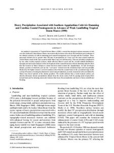
In OPER and TROP perturbations are applied to an extended tropical belt, and in consequence no perturbations are observed in latitudes beyond 308N and 458S. In OPER and EXT1, perturbations are on average almost half of those in other experiments (in Figs. 1a,c perturbations are scaled by 2). Since the same rescaling method and perturbation amplitude were used for all experiments, these differences in amplitude resulted from the application, or not, of perturbations to P and Q. Beyond differences in amplitude, experiments with and without perturbations on P and Q present significant differences with respect to the horizontal pattern. OPER and EXT1 produce similar perturbation in the tropical region (308S–308N). Intense perturbation centers can be observed over the three ocean basins and over Paraguay in South America. The center over South America seems to be associated with the constant low pressure observed in this region during the Southern Hemisphere summer. Near the equator, intense nuclei of perturbations over the Pacific and Indian Oceans seem to be related to the ITCZ and the action of the Asian monsoon, respectively. These patterns indicate that deep convection and release of latent heating during the model evolution have a preponderant role in the development of perturbations. Over the Atlantic, however, perturbations are elongated over almost the whole tropical ocean basin and seem not to be related to a synoptic system, except near the equator where the ITCZ could be having some influence. Over NH midlatitudes, EXT1 produces a maximum over the Pacific Ocean that resembles the region of maximum Eady index seen in Fig. 1f. Over SH midlatitudes, perturbations are smaller than those observed in NH and shifted equatorward of the latitudes where the maxima of the Eady index are observed. Experiments TROP, EXT2, and ETSA produce similar preferred regions for perturbation development, except for TROP over midlatitudes, where no perturbations are applied in this experiment. In contrast with the results of OPER and EXT1, over the tropics, perturbations are not spread through almost the whole region, but are more concentrated in regions with strong convective activity: northern South America and the western Pacific. In the subtropics of the Southern Hemisphere intense perturbations are observed, concentrated over regions in which large-scale condensation is important to the maintenance of the systems and represents a mode of interaction between the tropics and extratropics, by means of the two well-known systems that occur during Southern Hemisphere summer over the South Pacific and South Atlantic, called the South Pacific convergence zone (SPCZ) and the SACZ, respectively. These two phenomena are associated with the intense convective activity in the western Pacific and

APRIL 2009


1445

FIG. 1. January 2005 initial-time average for 500-hPa geopotential height. Ensemble mean (lines) and std dev (shading) for expts (a) OPER, (b) TROP, (c) EXT1, (d) EXT2, and (e) ETSA. (f) Absolute value of the Eady index. Contour interval (CI) is 5 m for ensemble std devs, and 0.2 day21 for the Eady index in (f). In (a) and (c), values of ensemble std devs are multiplied by 2.

northern South America and seem to dominate the development of EOF perturbations over the tropics/ subtropics of the Southern Hemisphere. These two preferred regions for EOF perturbation developments coincide with regions pointed out in earlier studies (Kalnay et al. 1986; Grimm and Silva Dias 1995) as sources of disturbances for many other regions around the globe through the propagation of Rossby wave trains that will influence the atmospheric regime in remote regions.

Over NH midlatitudes, EXT2 and ETSA show three preferred regions for perturbation development: the western and central North Pacific, eastern North America, and the western North Atlantic and northern Europe. Examining the Eady index (Fig. 1f) we observe that those preferred regions for perturbation development are close to regions with relative larger instability, suggesting that EOF perturbations are associated with baroclinic instability. Over SH midlatitudes, two centers of relatively intense perturbations appear around 1208E

1446


and 1208W. Both of these preferred regions are close to the areas of relative maxima of the Eady index, suggesting again that EOF perturbations in midlatitudes are related to baroclinic instability. Buizza et al. (2005) compared the performance of ECMWF, Meteorological Service of Canada (MSC), and NCEP ensembles over the Northern Hemisphere. Although the period is different from that used here (they present the average characteristics of the three ensembles for May 2002), it may be useful to do a qualitative comparison between their results and the results of the EOF method. In terms of the average value of ensemble spread it is observed that the EOF method produces approximately the same order of magnitude, around 30 m, over midlatitudes in the experiments TROP, EXT2, and ETSA, that they found for MSC and NCEP ensembles. However, the EOF method does not produce relatively strong perturbations over the polar region, as observed in MSC EPS and NCEP EPS. It is worth mentioning that the ensemble spread at initial time is strongly dependent on the amplitude of the perturbation rescaling. The spatial pattern of the initial perturbations is a more relevant characteristic to be compared. In midlatitudes, EOF perturbations preferentially developed close to regions of maximum Eady index. This characteristic is also observed for the ECMWF EPS. The geographical distribution of spread in each experiment at 2-day lead time was also computed (figure not shown) and compared with results of Buizza et al. (2005). Results indicate that extratropical EOF perturbations and perturbations on P and Q significantly increase the growth rate of the ensemble spread in midlatitudes. Nevertheless, the ensemble spread of CPTEC EPS exhibits lower growth rate than those of the ECMWF, NCEP, and MSC EPSs. After a general discussion based on the average characteristics of the EOF perturbations, a randomly selected case (1200 UTC 20 January 2005) is used to better investigate the main effects of using different configurations in the EOF method (in each experiment) on the dynamic structure of the EOF-based perturbations. The area considered in this evaluation is centered in midlatitudes over the South Atlantic Ocean. Figure 2 depict the synoptic systems that were acting at that time. At the surface a cyclone is observed (located near 508W and 428S with minimum MSLP of around 990 hPa) and part of a larger anticyclone in the top-right corner of Fig. 2a. In general, the associated circulation presents an approximate geostrophic balance. The cyclone is projected through the vertical almost without any tilt, as indicated by the geopotential height at 500 (Fig. 2b) and 250 hPa (Fig. 2c), which show a configuration typical of a barotropic system. The subtropical jet at the 250-hPa

VOLUME 137

FIG. 2. Overview of the randomly selected initial state for 1200 UTC 20 Jan 2005 over the South Atlantic Ocean: (a) MSLP (hPa) and 1000-hPa wind vector (m s21), (b) 500-hPa geopotential height (m, contours) and Eady index (day21, shading), and (c) 250-hPa geopotential height (m) and wind vector (m s21). CI is 0.3 day21 for the Eady index in (b). The reference for wind magnitude is indicated below (a) and (c).

pressure level is also observed acting over the northernmost part of the region considered, producing a relatively intense vertical wind shear. As a consequence, this region is identified as presenting a relatively high baroclinicity according to the Eady index, which can be identified at around 208–158W and 458S in Fig. 2b, with an absolute maximum of about 0.9 day21.

APRIL 2009


1447

FIG. 3. The 1200 UTC 20 Jan 2005 initial EOF perturbations of surface pressure and wind vector obtained from the difference time series between the control forecast and the random forecast started from the first randomly perturbed initial condition (n 5 1, see section 2c), for the following experiments: (a) OPER, (b) TROP, (c) EXT1, (d) EXT2, and (e) ETSA. Contour interval is 1 hPa for surface pressure. The reference for wind magnitude is indicated below the panels.

Since the EOF perturbations are computed separately for each analysis field, an important issue is whether these perturbations are balanced with each other. This point is addressed in Fig. 3, where the first EOF perturbations of the wind field at 1000 hPa are superimposed on perturbations of surface pressure for each experiment. Experiments OPER and EXT1 do not have perturbations on P and Q, so no contours of P perturbations appear in Figs. 3a,c. Weak wind perturbations are observed for OPER and EXT1 along with a poorly organized horizontal perturbation pattern

mainly in OPER; in EXT1 a small cyclonic region appears near the top-right corner of Fig. 3c. When perturbations are additionally computed for P and Q over the region ETR, a zonally elongated perturbation region centered around 308W and near the boundary of the perturbation domain (458S), is produced for surface pressure (Fig. 3b). This main perturbation has a maximum negative amplitude of around 24 hPa. From geostrophic theory, negative perturbations will induce cyclonic circulation around them. Wind perturbations are slightly enhanced when compared with perturbations

1448


in OPER and it can be seen that the cyclonic circulation is tied to the perturbations on P, with an almost geostrophic balance. When perturbations are computed as extratropical EOFs, we observe that the disturbances extend southward over a large area, reaching around 528S (Fig. 3d). Perturbation amplitudes are increased by around 26 hPa on P and 5 m s21 on wind. Two less intense nuclei of positive perturbations on P are observed near longitude 458W. Again, we can notice that wind perturbations are approximately geostrophic and present cyclonic circulation over negative perturbations and anticyclonic rotation over positive perturbations. For the analyzed region for this case, the target EOF perturbations over South America contribute to slightly diminish the perturbation amplitudes (Fig. 3e), however the horizontal pattern remains almost the same as that observed in EXT2. The results indicate that although no constraint is imposed on the perturbations and they have been computed separately for each field, an approximate balance among them is obtained, mainly when perturbations are included to surface pressure and specific humidity. This result is derived from the fact that although the model integration is started from a randomly perturbed initial condition, the error field gets organized after some hours. By commencing the EOF analysis from hour 6, contamination due to random effects is avoided. Another relevant point to be investigated is the vertical structure of EOF perturbations, which can reveal some hints about the nature of perturbations and mechanisms for perturbation growth. For this purpose, a vertical cross section of the first EOF perturbation of meridional wind component (V) is presented for the selected case at 448S at the initial time (Fig. 4) and 458S at t 1 48-h forecast (Fig. 5). We find first that the perturbations of experiment OPER present the least organized vertical structure at the initial time (Fig. 4a). The corresponding configuration of the EOF method does not seem to be able to capture the main mechanisms of perturbation growth in midlatitudes. The extratropical perturbations of EXT1 (Fig. 4c) present discontinuous nuclei that show westward tilt with vertical, suggesting that at least in parts they are associated with baroclinic instability. When perturbations on P and Q are included (experiments TROP, EXT2, and ETSA) a structure more typical of baroclinic systems is verified in the perturbations. Except for the intensity (in EXT2 they are more intense), perturbations in these three last experiments maintain many similarities (Figs. 4b,d,e). Consistent with the surface perturbations in Figs. 3b,d,e, we can observe a branch of negative perturbations localized approximately between 258 and 108W near the surface that

VOLUME 137

extends up to around 200 hPa. A branch of positive perturbations is also observed in the west side of those negative perturbations. The westward tilt of perturbations in the vertical indicates a baroclinic structure, suggesting that this mechanism is associated with the EOF perturbation growth in midlatitudes. Nonlinear evolution of the EOF perturbations is presented in Fig. 5 for 48-h lead time. Less growth were found in experiment OPER. This is consistent with results presented earlier in Fig. 4, since this experiment had less-organized initial perturbations. A positive maximum in the perturbations is observed close to 208–108W in OPER, extending from the surface up to around 200 hPa. In EXT1, perturbations are more intense than in OPER and a branch of negative perturbations can be observed close to 108W. Applying perturbations to P and Q, it is noticed that perturbations acquire more organized vertical structure. In experiments TROP, EXT2, and ETSA, positive perturbations are observed between 258 and 158W and a branch of negative perturbations is observed around 108W–08 (Figs. 5b,d,e). As expected, the domain in which initial perturbations are applied plays a significant role in the growth rate of the forecast perturbations. When the extratropics are disturbed (experiments EXT2 and ETSA) perturbations grow faster than in the case in which perturbations are applied only over the extended tropics (TROP). For this particular case, perturbations of EXT2 grow faster than in any other experiment. In all experiments, the westward tilt of initial perturbations was reduced after the 48-h nonlinear evolution and forecast perturbations acquire a barotropic structure. This behavior is similar to that pointed out by Randel and Stanford (1985) for the life cycle of mediumscale waves in the midlatitudes in the Southern Hemisphere summer: baroclinic growth in the initial stages and barotropic decay, with loss of energy to the zonal mean flow. These results are also similar to those found by Hoskins et al. (2000) and Coutinho et al. (2004) for the growth of ECMWF extratropical singular vectors.

b. Performance of the ensemble experiments based on statistical scores The performance of the control forecast was compared to the performance of experiment OPER to assess the advantages that operational CPTEC EPS forecasts have relative to control forecasts in a deterministic sense. Aiming to investigate the impact of modifications in the initial perturbation procedure of each experiment upon the performance of CPTEC EPS, we analyze the results according to two main sets of configurations of the procedure for the generation of the perturbed initial conditions. Investigated first are the

APRIL 2009


1449

FIG. 4. The 1200 UTC 20 Jan 2005 lon–pressure cross sections of EOF perturbations at 448S for meridional wind at initial time, obtained from the difference time series between the control forecast and the random forecast started from the first randomly perturbed initial condition (n 5 1, see section 2c), for the following expts: (a) OPER, (b) TROP, (c) EXT1, (d) EXT2, and (e) ETSA. The CI is 1 m s21.

1450


VOLUME 137

FIG. 5. Lon–pressure cross sections of 48-h nonlinear evolution for the meridional wind perturbations presented in Fig. 4, but at 458S, obtained as the difference between the 48-h forecasts started from the control initial condition (CIC) and the perturbed initial condition in which the EOF-based perturbations presented in Figs. 3–4 were added to the CIC. The time of control initial condition is 1200 UTC 20 Jan 2005. For the following expts: (a) OPER, (b) TROP, (c) EXT1, (d) EXT2 and (e) ETSA.

APRIL 2009


1451

FIG. 6. The 15 Dec 2004–15 Feb 2005 average pattern anomaly correlation (PAC) for the deterministic (DET, solid black lines) and the ensemble mean forecasts for experiments OPER (solid gray lines), TROP (short dashed lines), EXT1 (dotted lines), EXT2 (long dash–dotted lines), and ETSA (long dashed lines). Values refer to the 500-hPa geopotential height over the following regions: (a) NH, (b) SH, and (d) South America; and (c) for 850-hPa zonal wind component over the tropics. Vertical bars indicate the statistical errors for a confidence level of 90%, for experiment OPER.

impact of including perturbations to surface pressure and specific humidity fields, and the extension of EOF-based perturbations to the extratropics. After that, the impact of computing regional perturbations over South America is assessed. For brevity, over the tropics only the results of U850 will be presented, since V850 shows rather similar results and analogous conclusions are obtained for both.

1) CONTROL VERSUS ENSEMBLE MEAN FORECASTS

For a crude idea of benefits that EPS adds to the performance of CPTEC forecasts, the pattern anomaly correlation and rmse of the control forecast (CF) were computed and presented as thin, solid black lines in Figs. 6 and 7 . In Fig. 6, the error bars for a confidence level of 90% of experiment OPER are shown for each

1452


VOLUME 137

FIG. 7. The 15 Dec 2004–15 Feb 2005 average rmse of the ensemble mean forecasts (thick lines) and ensemble std dev (thin lines) for expts OPER (solid lines), TROP (short dashed lines), EXT1 (dotted lines), EXT2 (long dash–dotted lines), and ETSA (long dashed lines). The thin, solid black lines represent the average rmse of the DET. Values refer to the 500-hPa geopotential height over the following regions: (a) NH, (b) SH, and (d) South America; and for 850-hPa zonal wind component over the tropics in (c).

lead time. The error bars of other experiments are similar to those of OPER so they were omitted. The PAC values indicate that the ensemble mean (EM) is better than CF, except only for the two first lead times over NH and SH, and for the first four lead times over SA. Over SA, for the 7-day forecasts, PAC values

are 0.572 and 0.561 for EM and CF, respectively. It is also observed that in the sample used it is not possible discriminate between the pattern anomaly correlation of these two forecasts with a 90% confidence level. When rmse is considered, it is evident that the EM outperforms the control forecast in all regions and at all lead times,

APRIL 2009


1453

FIG. 8. The 15 Dec 2004–15 Feb 2005 average BSS for experiments OPER, TROP, EXT1, EXT2, and ETSA. Values have been computed considering the probability intervals according to the number of ensemble members and refer to the 500-hPa geopotential height over the following regions: (a) NH, (b) SH, and (d) South America; and (c) for 850-hPa zonal wind component over the tropics.

with the most significant improvements observed for U850 over the tropics. For lead time 10 over the TR, indices are 4.48 and 5.21 for EM and CF, respectively, which represents an improvement of almost 14%. The results obtained here are consistent with those presented in Buizza et al. (2005) for May–July 2002 over the NH for the ECMWF, MSC, and NCEP operational ensembles and those presented in Toth and Kalnay (1997) for 6 May–14 June 1992 over the NH, SH, and the tropics for the NCEP operational ensemble. It is important to emphasize that the two works cited are used as just a rough reference because they use different periods and different ensemble sizes.

2) IMPACT OF COMPUTING ADDITIONAL EOF-BASED PERTURBATIONS FOR THE EXTRATROPICS AND FOR SURFACE PRESSURE AND SPECIFIC HUMIDITY FIELDS

In this subsection, the impact on the CPTEC EPS of computing additional EOF-based perturbations for the extratropics and for surface pressure and specific humidity fields is discussed. These modifications were considered individually or combined in experiments OPER, TROP, EXT1, and EXT2. Three statistical scores (i.e., PAC, rmse, and spread) for these experiments are shown for all evaluated re-

gions in Figs. 6 and 7. The results of all experiments are analyzed and compared with each other. Assessing the quality of ensemble mean and ensemble spread, we notice that maintaining the operational perturbation region and including perturbations to P and Q fields (experiment TROP) yields ensemble forecasts that perform better than the operational version, mainly over NH. For this region at lead time 8, the anomaly correlation values are 0.550 for OPER against 0.560 for TROP, and the corresponding rmse (spread) values are 104.95 (33.62) for OPER and 103.75 (34.48) for TROP. Over other regions, the results show a slight tendency for TROP to be better than OPER but this is not true for all lead times; for example, over SA at lead time 7 the spread of TROP (12.94) is smaller than OPER (13.04). The results of PAC are not significant when compared with the 90% confidence level error bars. Perturbations to P and Q fields improve the probabilistic forecasts of EPS. The BSS index is presented in Fig. 8. It is observed that BSS is especially increased for the tropics and SA regions, mainly for lead times beyond 2. The components of the BSS are shown in Tables 3–6. For the four evaluated experiments, the best indexes are highlighted in boldface. When indexes are similar for more than one experiment, all of them are highlighted. In general, RES is greater and REL is smaller for TROP.

1454


VOLUME 137

TABLE 3. Average REL and RES (values in parentheses) contributions to BSS for all expts (columns) and for all forecast lead time (rows). Values have been computed considering the probability intervals according to the number of ensemble members. Values refer to 500-hPa geopotential height field over NH. For each lead time, boldface signifies the best value among experiments OPER, TROP, EXT1, and EXT2. Italics signifies the best result between experiments EXT2 and ETSA. Values are multiplied by a factor of 102. Expt Forecast lead time (days)

OPER

TROP

EXT1

EXT2

ETSA

1 2 3 4 5 6 7 8 9 10

0.449 (16.834) 1.254 (13.240) 2.055 (10.716) 3.140 (8.252) 4.422 (5.961) 5.399 (4.310) 4.855 (3.849) 4.421 (3.499) 4.226 (2.918) 4.000 (2.374)

0.399 (16.995) 0.997 (14.378) 1.760 (11.573) 2.741 (8.970) 4.284 (6.013) 5.234 (4.413) 4.620 (3.990) 4.162 (3.589) 4.185 (2.856) 3.999 (2.324)

0.280 (17.940) 0.843 (14.595) 1.255 (12.455) 1.846 (10.029) 2.599 (7.411) 2.824 (6.094) 2.810 (4.902) 2.888 (3.974) 2.866 (3.240) 2.702 (2.705)

0.151 (18.491) 0.544 (15.790) 0.951 (13.165) 1.494 (10.330) 2.204 (7.536) 2.226 (6.458) 2.348 (5.021) 2.570 (3.917) 2.614 (3.120) 2.486 (2.583)

0.164 (18.353) 0.537 (15.805) 0.974 (13.019) 1.489 (10.353) 2.213 (7.533) 2.259 (6.409) 2.384 (4.986) 2.593 (3.883) 2.617 (3.116) 2.493 (2.577)

Over SA at lead time 7, REL (RES) are 5.648 (3.481) for OPER and 3.837 (5.351) for TROP, which indicates an improvement for probabilistic forecasts. PECA values indicate that extra initial perturbations to P and Q in experiment TROP do not provide significant diversity to forecast perturbations over the extratropics (NH and SH) and SA, since indices are similar for OPER and TROP (Figs. 9a,b,c). Over the tropics (Fig. 9c), the impact is slightly positive, mainly for lead times longer than 3 days when individual perturbations are considered. In experiment EXT1 the extension of EOF-based perturbations to the extratropics is tested. The application of these extra perturbations has a positive impact on the NH and SH regions (Figs. 6a,b and 7a,b). The ensemble mean of EXT1 performs better than OPER for all lead times. Over NH, the ensemble spread of EXT1 is almost double that of OPER for lead time 1 (7.35 against 3.97). For U850, over the tropics (Figs. 6c and 7c), PAC and rmse are not much affected, but spread is diminished for lead times beyond 6. Over SA (Figs. 6d and 7d), the ensemble spread is increased, but

in terms of PAC and rmse the EXT1 ensemble mean performs better mainly for lead times beyond 6. In terms of probabilistic forecasts, greater positive effects are observed again over NH and SH (Figs. 8a,b and Tables 3 and 4). The impact on TR is approximately neutral according to BSS. Probabilistic forecasts are slightly better over SA (Fig. 8d) and it can be seen that the main contribution comes from improvements in the forecast reliability (Table 6). It is evident that perturbations in the extratropics, represented by the dotted lines in Fig. 9, have a significant impact on the quality of the forecast perturbations over NH and a slight impact over SH and SA. Over the tropics, impact is slightly negative. This is probably the reason for the adverse results obtained for the quality of ensemble forecasts over TR in EXT1. Results of EXT1 show that forecasts over extratropical regions are improved when extratropical EOF-based perturbations are computed, which means that more spread and variety are incorporated in the forecasts when these extra perturbations are included in the initial conditions. Moreover, midlatitudes yield the best results. As

TABLE 4. As in Table 3, but for the SH. Expt Forecast lead time (days)

OPER

TROP

EXT1

EXT2

ETSA

1 2 3 4 5 6 7 8 9 10

0.278 (18.934) 0.692 (15.534) 1.487 (11.941) 2.479 (8.654) 3.233 (6.361) 3.707 (4.841) 3.859 (3.802) 4.050 (2.931) 4.617 (1.977) 5.192 (1.208)

0.322 (19.100) 0.558 (16.280) 1.206 (12.905) 2.179 (9.318) 2.954 (6.900) 3.509 (5.265) 3.789 (4.075) 4.071 (3.031) 4.443 (2.134) 5.204 (1.275)

0.257 (19.080) 0.673 (15.834) 1.417 (12.392) 2.424 (8.780) 3.005 (6.628) 3.553 (4.903) 3.697 (3.847) 3.927 (2.955) 4.467 (2.008) 4.929 (1.211)

0.186 (19.410) 0.427 (16.734) 0.975 (13.333) 1.810 (9.729) 2.529 (7.180) 2.987 (5.495) 3.374 (4.191) 3.636 (3.149) 4.027 (2.185) 4.756 (1.305)

0.246 (19.223) 0.417 (16.825) 0.938 (13.476) 1.720 (10.056) 2.522 (7.305) 2.911 (5.724) 3.317 (4.329) 3.359 (3.439) 3.688 (2.476) 4.302 (1.568)

1455


APRIL 2009

TABLE 5. As in Table 3, but for the tropics. Expt Forecast lead time (days)

OPER

TROP

EXT1

EXT2

ETSA

1 2 3 4 5 6 7 8 9 10

1.062 (3.968) 1.879 (2.532) 2.858 (1.632) 4.017 (1.046) 4.684 (0.687) 5.165 (0.417) 5.701 (0.235) 5.771 (0.161) 5.800 (0.108) 5.697 (0.109)

0.909 (4.008) 1.274 (2.711) 2.438 (1.653) 3.451 (1.057) 4.161 (0.664) 4.526 (0.403) 4.828 (0.220) 5.026 (0.142) 5.007 (0.089) 5.120 (0.063)

1.006 (4.088) 1.928 (2.598) 2.861 (1.633) 3.992 (1.062) 4.694 (0.688) 5.081 (0.421) 5.486 (0.226) 5.539 (0.144) 5.498 (0.120) 5.277 (0.101)

0.837 (4.173) 1.328 (2.804) 2.326 (1.680) 3.291 (1.096) 3.992 (0.676) 4.102 (0.440) 4.518 (0.238) 4.707 (0.163) 4.692 (0.110) 4.629 (0.109)

0.843 (4.165) 1.330 (2.801) 2.324 (1.682) 3.290 (1.098) 3.991 (0.678) 4.108 (0.431) 4.526 (0.235) 4.704 (0.160) 4.681 (0.119) 4.623 (0.104)

presented in Fig. 1c, initial EOF perturbations of EXT1 in midlatitudes are concentrated close to regions with higher baroclinicity as measured by the Eady index (Fig. 1f). Since baroclinic instability is the main mechanism responsible for synoptic system development in midlatitudes then this suggests that the EOF-based method is able to capture part of that mechanism of perturbation growth. The computation of unstable modes on a more restricted belt (208N–208S) seems to have eliminated some important characteristics for perturbation growth in the tropics. Eliminating the subtropics from the computation of tropical-EOF perturbations may have inhibited the influence of tropic–extratropic interactions, which should have affected the development of perturbations. As found in the experiments TROP and EXT1, separate EOF-based perturbations in the extratropics and on P and Q fields have, in general, positive impact on the performance of CPTEC EPS mainly over the tropics and midlatitudes, respectively. In experiment EXT2, the impact on the ensemble performance of using a combination of these two modifications in the perturbation method configuration is investigated. The quality of the ensemble mean and the ensemble spread is enhanced over all verification regions for most

of the lead times (Figs. 6 and 7). Over NH at lead time 7, the rmse (spread) are 97.79 (26.97) for OPER and 93.46 (40.00) for EXT2. It is clear that the most significant impact is on ensemble spread, which increases by a factor of almost 2 in this case. Improvements in the ensemble spread contribute to produce more balanced probability forecasts, which can be noticed through their effect on the reduction of the probabilistic forecast reliability (REL; Tables 3–6) for almost all lead times. The capacity to discern subsample forecast periods with different relative frequencies of the event was also improved. The RES values in EXT2 are larger than in experiments OPER, TROP, and EXT1; for example, at lead time 7 over SH, values are 3.802 for OPER and 4.191 for EXT2. The BSS (Fig. 8) also indicates that better probabilistic forecasts are produced combining additional EOF-based perturbations in the extratropics and on P and Q fields with tropical EOF-based perturbations. PECA of EXT2 (long dash–dotted lines in Fig. 9) indicates that combining perturbations in the extratropics with perturbations on P and Q fields is able to reproduce the individual improvements that were observed over particular regions when both modifications

TABLE 6. As in Table 3, but for South America. Expt Forecast lead time (days)

OPER

TROP

EXT1

EXT2

ETSA

1 2 3 4 5 6 7 8 9 10

0.043 (20.129) 0.580 (17.446) 1.466 (13.023) 1.844 (11.522) 2.180 (9.741) 3.608 (6.029) 5.648 (3.481) 5.183 (3.416) 4.606 (3.122) 6.628 (1.178)

0.107 (20.057) 0.307 (18.488) 0.920 (15.195) 1.157 (13.835) 1.529 (12.253) 2.501 (8.115) 3.837 (5.351) 3.779 (5.408) 3.986 (4.489) 5.698 (1.940)

0.041 (20.150) 0.544 (17.520) 1.467 (13.117) 1.808 (11.634) 2.189 (9.800) 3.562 (5.854) 5.865 (3.354) 4.947 (3.312) 4.512 (3.061) 6.413 (1.144)

0.109 (20.092) 0.266 (18.551) 0.783 (15.489) 0.988 (14.239) 1.342 (12.456) 2.228 (8.216) 3.614 (5.323) 3.459 (5.344) 3.612 (4.363) 5.157 (2.090)

0.365 (19.727) 0.130 (18.843) 0.650 (16.121) 0.803 (14.667) 1.168 (12.619) 2.086 (8.437) 3.355 (5.568) 3.379 (5.571) 3.261 (4.867) 4.321 (2.795)

1456


VOLUME 137

FIG. 9. The 15 Dec 2004–15 Feb 2005 average correlation between control forecast error and ensemble perturbations for expts OPER, TROP, EXT1, EXT2, and ETSA. Thin lines represent values averaged over 14 individual ensemble perturbations (sin), while thick lines represent values for an optimal combination of the individual perturbations (opt). Values refer to the 500-hPa geopotential height over the following regions: (a) NH, (b) SH, and (d) South America; and (c) for multivariate three-dimensional field (U, V, T) at 850, 500, and 250-hPa, respectively, over the tropics.

are applied separately in experiments TROP and EXT1. Thus, the combination of those extra initial perturbations seemed to create more diversity in the initial perturbation patterns, which contributed to the improvement of the variance of the forecast error explained by ensemble perturbations. The results presented in this subsection are in agreement with results of section 3a (i.e., applying perturbations to P and Q and extending those perturbations to the extratropics contributes to the generation of bettersuited initial perturbations and consequently improved

ensemble forecasts). The results also indicate that the underdispersion of the system is alleviated, although in spite of this it remains underdispersive. A rough qualitative comparison of these results with those of Buizza et al. (2005; they use a different period and a smaller number of members) reveals that, in terms of rmse and spread in midlatitudes, the CPTEC EPS presents less balance between the growth of rmse and spread, indicating that it is more underdispersive. It is remembered that they found that the ECMWF, MSC, and NCEP EPSs showed underdispersion only for lead times

APRIL 2009


beyond 5, 4, and 4 days, respectively. In terms of quality of probabilistic forecasts, BSS of the CPTEC EPS presented positive values approximately up to the same range that was found by Buizza et al. (2005) over midlatitudes for ECMWF, MSC, and NCEP ensembles, around a lead time of 6 or 7 days. Wei and Toth (2003) compared the quality of perturbation patterns of the ECMWF and NCEP EPSs using PECA for April 2001. Wei et al. (2006) also used PECA to study the correlation between ensemble perturbations and forecast errors for two methods of producing initial perturbations with NCEP global forecasting system: breeding of growing modes and a version of an ensemble transform Kalman filter. In this case the period used was 15 January–15 February 2003. Over midlatitudes, the PECA values obtained with the EOF method are qualitatively comparable to those shown in Wei and Toth (2003) and Wei et al. (2006). In general, it is observed that the PECA values increase with increasing lead time. This is related to the convergence of both the perturbation and the error patterns to a small subspace of growing patterns (Wei and Toth 2003). Over the tropics, the PECA obtained with the EOF method for the three-dimensional variable p(U, V, T ) presents a behavior similar to those found by Wei and Toth (2003), though values are closer to those exhibited by the ECMWF EPS.

3) IMPACT OF REGIONAL COMPUTED OVER SA

PERTURBATIONS

The impact of including regional perturbations over the South America region is assessed in this subsection. In experiment ETSA, besides the extension of initial perturbations to the extratropics and the inclusion of perturbations on P and Q fields, two South America subregions are considered in order to compute regional perturbations: NSA (208S–208N, 1008–108W) and SSA (608–208S, 1108–208W). The results of EXT2 are used as a reference for evaluating ETSA, since they were produced from a similar configuration of the initial perturbation method, except with additional regional perturbations over SA in ETSA. In terms of quality of ensemble mean and ensemble spread, including new regional perturbations does not have significant impact over NH (Figs. 6a and 7a). Over SH (Figs. 6b and 7b) there is a slight positive impact on EM, but not on spread. For U850, over the tropics (Figs. 6c and 7c), PAC, rmse, and spread values are approximately the same as in EXT2 for all lead times. The main purpose of this experiment is to attempt to produce better forecasts over SA. Looking at the indices for SA (Figs. 6d and 7d), it is observed that at many of the lead

1457

times, ETSA is more skillful than EXT2. For lead time 7, the rmse (spread) are 53.41 (14.09) for EXT2 against 52.98 (14.29) for ETSA. Consistent with the results obtained for quality of the ensemble mean, probabilistic forecasts are not improved over NH (Fig. 8a and Table 3). In contrast, over SH, BSS, and RES increased while REL diminished for almost all lead times (Fig. 8b and Table 4). Probabilistic forecasts over TR are enhanced in relation to OPER, but in relation to EXT2 similar statistical scores were found for U850 (Fig. 8c and Table 5). Over SA, probabilistic forecasts are enhanced by the new regional perturbations (Fig. 8d and Table 6), at lead time 7, REL (RES) are 3.614 (5.323) for EXT2 and 3.355 (5.568) for ETSA. PECA for ETSA reveals a smaller impact over the extratropics (NH and SH). However, extra perturbations over SA clearly contribute to the improvement of the fraction of forecast error explained by perturbation forecasts over the tropics and SA. Over TR, at lead time 10 for combined perturbations (thick long-dashed line of Fig. 9c), the correlation increases from around 0.46 in EXT2 to around 0.49 in ETSA. The impact of the regional perturbations of experiment ETSA is more significant over regions TR and SA, which suggests that local EOF-based perturbations are able to capture initial uncertainties associated with small scales and can be used to improve the perturbation growth over the target regions.

4. Discussion and conclusions The effect of using the EOF method to insert extra initial perturbations in the extratropics and surface pressure and specific humidity fields in the CPTEC/ INPE EPS was addressed in this study. Also, the computation of regional perturbations over South America was studied. Under the perfect-model hypothesis, five experiments were performed by modifying the regions used to compute the initial perturbations and applying perturbations to the P and Q fields. The impact of such changes was assessed analyzing the structure of the EOF-based perturbations and using statistical scores to measure the quality of the forecasts in each experiment over a 2-month period, from 15 December 2004–15 February 2005. Our results showed that extratropical EOF-based perturbations develop preferentially near regions with high baroclinicity in midlatitudes and close to areas of important synoptic systems that act in the tropics– extratropics of the Southern Hemisphere during the austral summer. We also found that additional perturbations on P and Q are important in obtaining perturbations that are more spatially organized and with more

1458


baroclinic structures in midlatitudes. This modification also seems to produce perturbations that grow faster than in those cases in which no perturbations are applied to P and Q, during the nonlinear model integration. Consistent with these results, statistical evaluation indicates that extratropical EOF-based perturbations span a subspace in the phase space representing fast-growing errors, contributing to the enhancement of the ensemble forecast quality in both a deterministic and probabilistic sense and, moreover, including more diversity in the CPTEC EPS initial perturbations. These extra perturbations have a positive effect on EPS performance, mainly over the extratropics. Perturbations to P and Q fields allow the inclusion of more diversity in the initial perturbations and produce an improvement of the ensemble forecast quality mainly over the tropics. The combination of these two extra perturbations is able to reproduce the main positive effects that are observed when each one is applied individually, and proved to be a more suitable configuration for the initial perturbation method. Regional EOF-based perturbations computed separately over northern South America and southern South America in addition to hemispheric perturbations contributed in a general sense to the improvement of local forecasts over the target region. Overall, the application of the EOF method to perturb midlatitude variables, including surface pressure and specific humidity fields, produced positive impact on the quality of CPTEC EPS and alleviated the underdispersion of the system. We suggest that part of this CPTEC EPS underdispersion is associated with rapid error growth in the CPTEC AGCM in the first 24 h of model integration due to two main reasons: starting the integration with an analysis that is not produced by the same model and the presence of deficiencies in physical parameterizations. Therefore, we intend to investigate, in future work, the influence that perturbations in physical processes have on the quality of CPTEC/INPE ensemble forecasts, as has been done operationally at MSC and ECMWF. The use of control analyses created by CPTEC AGCM itself to generate EOF-perturbed initial conditions will be also investigated. Currently, a data assimilation cycle based on the Physical-space Statistical Analysis System (Cohn et al. 1998) associated with the CPTEC AGCM is running in a parallel operational suite. The implementation of a local ensemble Kalman filter (Ott et al. 2004) version for data assimilation and ensemble forecasting is in progress at CPTEC/INPE and should also be evaluated. The results of this study encourage an operational implementation of additional EOF-based perturbations in the extratropics and on P and Q fields, as well as, regional perturbations over South America at CPTEC

VOLUME 137

EPS in order to improve the quality of CPTEC/INPE ensemble forecasts. Acknowledgments. We thank Dr. T. N. Krishnamurti and Dr. Z. Zhang from The Florida State University (FSU) for providing the original computational procedures of the EOF method. We also thank Dr. M. M. Coutinho for her effort in adapting the original procedures of the EOF method for the CPTEC AGCM and her helpful support during the operational implementation of the CPTEC EPS. Thanks are also given to Dr. Peter Caplan, for going through the manuscript, and to the anonymous reviewers for their suggestions.

REFERENCES Anderson, J. L., B. Wyman, S. Zhang, and T. Hoar, 2005: Assimilation of surface pressure observations using an ensemble filter in an idealized global atmospheric prediction system. J. Atmos. Sci., 62, 2925–2938. Barkmeijer, J., R. Buizza, T. N. Palmer, K. Puri, and J.-F. Mahfouf, 2001: Tropical singular vectors computed with linearized diabatic physics. Quart. J. Roy. Meteor. Soc., 127, 685–708. Bishop, C. H., B. J. Etherton, and S. Majumdar, 2001: Adaptive sampling with the ensemble transform Kalman filter. Part I: Theoretical aspects. Mon. Wea. Rev., 129, 420–436. Buizza, R., M. J. Miller, and T. N. Palmer, 1999: Stochastic simulation of model uncertainties in the ECMWF Ensemble Prediction System. Quart. J. Roy. Meteor. Soc., 125, 2887– 2908. ——, P. L. Houtekamer, Z. Toth, G. Pellerin, M. Wei, and Y. Zhu, 2005: A comparison of the ECMWF, MSC, and NCEP Global Ensemble Prediction Systems. Mon. Wea. Rev., 133, 1076– 1097. Cohn, S. E., A. Silva, J. Guo, M. Sienkiewicz, and D. Lamich, 1998: Assessing the effects of data selection with the DAO physicalspace statistical analysis system. Mon. Wea. Rev., 126, 2913– 2926. Coutinho, M. M., 1999: Previsaõ por conjuntos utilizando perturbac xo˜es baseadas em componentes principais (Ensemble prediction using principal-component-based perturbations). M.S. dissertation, Brazilian National Institute for Space Research (INPE), S. J. Campos, SP, Brazil, 136 pp. ——, B. J. Hoskins, and R. Buizza, 2004: The influence of physical processes on extratropical singular vectors. J. Atmos. Sci., 61, 195–209. Daley, R., and T. Mayer, 1986: Estimates of global analysis error from the global weather experiment observational network. Mon. Wea. Rev., 114, 1642–1653. Derber, J., and F. Bouttier, 1999: A reformulation of the background error covariance in the ECMWF Global Data Assimilation System. Tellus, 51A, 195–221. Farina, L., A. M. Mendoncxa, and J. P. Bonatti, 2005: Approximation of ensemble members in ocean wave prediction. Tellus, 57A, 204–216. Grimm, A. M., and P. L. Silva Dias, 1995: Analysis of tropical– extratropical interactions with influence functions of a barotropic model. J. Atmos. Sci., 52, 3538–3555.

APRIL 2009


Hamill, T. M., 2002: Ensemble-based data assimilation. Proc. Seminar on Predictability of Weather and Climate, Reading, United Kingdom, ECMWF, 83–105. ——, C. Snyder, and J. S. Whitaker, 2003: Ensemble forecasts and the properties of flow-dependent analysis-error covariance singular vectors. Mon. Wea. Rev., 131, 1741–1758. Holton, J. R., 2004: An Introduction to Dynamic Meteorology. 4th ed. Elsevier Academic Press, 535 pp. Hoskins, B. J., and J. Karoly, 1981: The steady linear response of a spherical atmosphere to thermal and orographic forcing. J. Atmos. Sci., 38, 1179–1196. ——, and P. J. Valdes, 1990: On the existence of storm-tracks. J. Atmos. Sci., 47, 1854–1864. ——, R. Buizza, and J. Badger, 2000: The nature of singular growth and structure. Quart. J. Roy. Meteor. Soc., 126, 1565– 1580. Houtekamer, P. L., L. Lefaivrem, J. Derome, H. Ritchie, and H. L. Mitchell, 1996: A system simulation approach to ensemble prediction. Mon. Wea. Rev., 124, 1225–1242. ——, H. L. Mitchell, G. Pellerin, M. Buehner, M. Charron, L. Spacek, and B. Hansen, 2005: Atmospheric data assimilation with an ensemble Kalman filter: Results with real observations. Mon. Wea. Rev., 133, 604–620. Kalnay, E., K. C. Mo, and J. Paegle, 1986: Large-amplitude, shortscale stationary Rossby waves in the Southern Hemisphere: Observations and mechanistic experiments to determine their origin. J. Atmos. Sci., 43, 252–275. ——, and Coauthors, 2002: Data assimilation via local ensemble Kalman filtering. Proc. Seminar on Predictability of Weather and Climate, Reading, United Kingdom, ECMWF, 41–45. Kanamitsu, M., W. Ebisuzaki, J. Woollen, S.-K. Yang, J. J. Hnilo, M. Fiorino, and G. L. Potter, 2002: NCEP-DEO AMIP-II Reanalysis (R-2). Bull. Amer. Meteor. Soc., 83, 1631–1643. Kinter, J. L., and Coauthors, 1997: Formulation. Vol. 1, The COLA atmosphere-biosphere general circulation model. COLA Rep. 51, COLA, 49 pp. Krishnamurti, T. N., C. M. Kishtawal, Z. Zhang, T. LaRow, D. Bachiochi, and E. Williford, 2000: Multimodel ensemble forecasts for weather and seasonal climate. J. Climate, 13, 4196–4216. Legler, D. M., 1983: Empirical orthogonal function analysis of wind vectors over the tropical Pacific region. Bull. Amer. Meteor. Soc., 64, 234–241. Liebmann, B., and D. L. Hartmann, 1984: An observational study of tropical–midlatitude interaction on intraseasonal time scales during winter. J. Atmos. Sci., 41, 3333–3350. Lorenz, E. N., 1963: Deterministic non-periodic flow. J. Atmos. Sci., 20, 130–141. ——, 1965: A study of the predictability of a 28-variable atmospheric model. Tellus, 17A, 321–333. ——, 1969: The predictability of a flow which possesses many scales of motion. Tellus, 21A, 289–307. Mendoncxa, A. M., and J. P. Bonatti, 2006: Experiments with EOFbased perturbation method to ensemble weather forecasting in midlatitudes. Proc. Eighth Int. Conf. on Southern Hemi-

1459

sphere Meteorology and Oceanography, Foz do Iguac xu, Brazil, INPE, 1829–1832. Mo, K. C., and R. W. Higgins, 1998: The Pacific–South American modes and tropical convection during the Southern Hemisphere winter. Mon. Wea. Rev., 126, 1581–1596. Molteni, F., R. Buizza, T. N. Palmer, and T. Petroliagis, 1996: The ECMWF Ensemble Prediction System: Methodology and validation. Quart. J. Roy. Meteor. Soc., 122, 73–119. Ott, E., and Coauthors, 2004: A local ensemble Kalman filter for atmospheric data assimilation. Tellus, 56A, 415–428. Palmer, T. N., 1988: Large-scale tropical, extratropical interactions on time-scales of a few days to a season. Aust. Meteor. Mag., 36, 107–125. Puri, K., J. Barkmeijer, and T. N. Palmer, 2001: Ensemble prediction of tropical cyclones using targeted diabatic singular vectors. Quart. J. Roy. Meteor. Soc., 127, 709–731. Rabier, F., H. Ja¨rvinen, E. Klinker, J.-F. Mahfouf, and A. Simmons, 2000: The ECMWF operational implementation of four-dimensional variational assimilation. I: Experimental results with simplified physics. Quart. J. Roy. Meteor. Soc., 126, 1143–1170. Randel, W. J., and J. L. Stanford, 1985: The observed life cycle of a baroclinic instability. J. Atmos. Sci., 42, 1364–1373. Reynolds, C. A., P. J. Webster, and E. Kalnay, 1994: Random error growth in NMC’s global forecasts. Mon. Wea. Rev., 122, 1281– 1305. Simmons, A. J., 1982: The forcing of stationary wave motion by tropical diabatic heating. Quart. J. Roy. Meteor. Soc., 108, 503–534. Toth, Z., and E. Kalnay, 1993: Ensemble forecasting at NMC: The generation of perturbations. Bull. Amer. Meteor. Soc., 74, 2317–2330. ——, and ——, 1997: Ensemble forecasting at NCEP and the breeding method. Mon. Wea. Rev., 125, 3297–3319. Wang, X., and C. H. Bishop, 2003: A comparison of breeding and ensemble transform Kalman filter ensemble forecast schemes. J. Atmos. Sci., 60, 1140–1158. Wei, M., and Z. Toth, 2003: A new measure of ensemble performance: Perturbation versus Error Correlation Analysis (PECA). Mon. Wea. Rev., 131, 1549–1565. ——, ——, R. Wobus, Y. Zhu, C. H. Bishop, and X. Wang, 2006: Ensemble transform Kalman filter-based ensemble perturbations in an operational global prediction system at NCEP. Tellus, 58A, 28–44. Wilks, D. S., 1995: Statistical Methods in the Atmospheric Sciences. Academic Press, 467 pp. WMO, 1992: Manual on the global data-processing system. WMO 485, 217 pp. Zhang, Z., 1997: Hurricane ensemble prediction using EOF-based perturbations. Ph.D. dissertation, Florida State University, Tallahassee, FL, 173 pp. ——, and T. N. Krishnamurti, 1999: A perturbation method for hurricane ensemble predictions. Mon. Wea. Rev., 127, 447– 469.

Experiments with EOF-Based Perturbation Methods ... - AMS Journals

Experiments with EOF-Based Perturbation Methods ... - AMS Journals

Suggest Documents

Observing System Simulation Experiments - AMS Journals - American ...

Observing System Simulation Experiments - AMS Journals - American ...

Perturbation Methods

Inverse Methods - AMS Journals - American Meteorological Society

Perturbation Methods - IEEE Xplore

Numerical Experiments of an Advanced Radiative ... - AMS Journals

Experiments on Differential Scalar Mixing in ... - AMS Journals

North American Climate in CMIP5 Experiments: Part III ... - AMS Journals

North American Climate in CMIP5 Experiments. Part I ... - AMS Journals

Observing System Experiments in a 3DVAR Data ... - AMS Journals

SST Assimilation Experiments in a Tropical Pacific ... - AMS Journals

Design and Analysis of Climate Model Experiments for ... - AMS Journals

Part 2: Experimental design of perturbation experiments

Experiments with Statistical Connectionist Methods and Hidden ...

CO perturbation experiments: similarities and differences between ...

CO2 perturbation experiments: similarities and differences between ...

Perturbation Experiments in Community Plant Species during ...

QuikSCAT Satellite Comparisons with Nearshore ... - AMS Journals

Heavy Precipitation Associated with Southern ... - AMS Journals

QUANTITATIVE METHODS IN CLASSICAL PERTURBATION ...

An Analogy with Monopulse Radar - AMS Journals

A Comparison of Methods for Determining Significant ... - AMS Journals

Application of Two Spatial Verification Methods to ... - AMS Journals

Underway and Moored Methods for Improving ... - AMS Journals