Explicit versus Implicit Graph Feature Maps: A ... - Semantic Scholar
Recommend Documents
either implicitly or explicitly on a distance or a similarity measure. Definition of .... between the lines i and j of X. Equation 1 may thus be intepreted as a classical.
Jun 13, 2013 - of the predictive sequence was implicit, while in the second this regularity was made explicit. ... Funding: This work was supported by the Spanish Ministry of ...... Barch DM, Carter CS, Braver TS, Sabb FW, MacDonald A, et al.
Abstract:The present study examined whether 1) placebo hypoalgesia can be generated through implicit associative learning (ie, conditioning in the absence of ...
Jun 13, 2013 - Both the implicit and explicit sessions showed shorter reaction times and peak P3b ..... lines indicate time of stimulus presentation onset.
May 12, 2005 - ranking implied from the partial WTP-values (Olsen and Donaldson, ..... Professor Michael Jones-Lee, University of Newcastle upon Tyne, UK.
This paper describes a representation for time relations in narrative. The time relations are based on both explicit sources of time information. (e.g., adverbial ...
ing the temporal offset, relies on explicit feature maps [23]. Compared to ...... 11. strokkur geyser 12. thailand flood 2011 13. universal studios jurassic park ride.
Stanoevska-slabeva and Wozniak , 2011). ..... Hennig-Thurau, T., Gwinner, K.P., Walsh, G. and Gremler, D.D. (2004) Electronic word-of-mouth via consumer-.
May 12, 2014 - Adorno TW, Frenkel-Brunswick E, Levinson DJ, Sanford RN (1950) The authoritarian personality. New York: Harper & Row. 3. Caprara GV ...
digm, a color name is presented in different ink colors (e.g., the word RED in red or .... a Windows 2000 desktop comput
a grapheme-color synesthete, who experiences colors when viewing digits but not ... despite the fact that NM denied experiencing colors for random dot patterns, ...... Campbell JI, Parker HR, and Doetzel NL. .... psyche-8-01-smilek.html, 2002.
clustering methods to a connectionist approach in the field of exploratory data analysis. Using an Artificial. Neural network, namely Kohonen's Self-Organizing.
University of Marburg. FG Neuroinformatik & Künstliche Intelligenz. Research Report 0994. Abstract. In this paper we oppose some classical statistical clustering ...
To explain this kind of implicit-explicit dissociation, some ... these lines, it has been shown that in AD the extrastriatal cortex â where reduced activation is.
May 28, 2018 - It is based on the combination of the explicit scheme, implicit ... signal processing and information recognition [1] [2] [3]. Due to the ... segment explicit-implicit (ASE-I) parallel difference method is constructed. The ...... the p
attitude formation when behavioral information about the target was ambiguous. ..... CA information are presented, implicit attitudes should eventually change in ...
Keywords: Implicit contracts, repeated games. JEL classification numbers: L14, C72, J33. Wirtschaftspolitische Abteilung, University of Bonn, Adenauerallee 24, ...
Apr 11, 2014 - Explicit and implicit timing activates different distributed brain networks. ..... represented with vertical dashed lines for the four different durations.
Event-related brain potentials (ERPs) were recorded during a serial reaction time (RT) task, where single deviant items seldom (Experiment 1) or frequently ...
May 22, 2000 - User Group, Mitel Corporation and Nortel Networks. I am also indebted towards my supervisor, Luigi Logrippo, and my former co-supervisor, ...
interactive iconic tool (Interactive-Icon) and floating text-based ... interface tools) for solving complex analytical problems (tasks) with a highly interactive visual ...
Explicit versus Implicit Graph Feature Maps: A ... - Semantic Scholar
A Computational Phase Transition for Walk Kernels. Nils Kriegeâ ... implicit computation is superior for longer walk lengths and data sets with larger label ...
Explicit versus Implicit Graph Feature Maps: A Computational Phase Transition for Walk Kernels Nils Kriege† , Marion Neumann∗ , Kristian Kersting† , Petra Mutzel† †
Dept. of Computer Science, TU Dortmund, Germany Email: {nils.kriege,kristian.kersting,petra.mutzel}@tu-dortmund.de ∗ BIT, University of Bonn, Germany Email: [email protected]
Abstract—As many real-world data can elegantly be represented as graphs, various graph kernels and methods for computing them have been proposed. Surprisingly, many of the recent graph kernels do not employ the kernel trick anymore but rather compute an explicit feature map and report higher efficiency. So, is there really no benefit of the kernel trick when it comes to graphs? Triggered by this question, we investigate under which conditions it is possible to compute a graph kernel explicitly and for which graph properties this computation is actually more efficient. We give a sufficient condition for Rconvolution kernels that enables kernel computation by explicit mapping. We theoretically and experimentally analyze efficiency and flexibility of implicit kernel functions and dot products of explicitly computed feature maps for widely used graph kernels such as random walk kernels, subgraph matching kernels, and shortest-path kernels. For walk kernels we observe a phase transition when comparing runtime with respect to label diversity and walk lengths leading to the conclusion that explicit computations are only favorable for smaller label sets and walk lengths whereas implicit computation is superior for longer walk lengths and data sets with larger label diversity.
I. I NTRODUCTION Analyzing complex data is becoming more and more important. In numerous application domains, e.g., chem- and bioinformatics or image and social network analysis, the data is structured and hence can naturally be represented as graphs. To achieve successful learning we need to exploit the rich information inherent in the graph structure and the annotations of nodes and edges. A popular approach to mining structured data is to design graph kernels measuring the similarity between graphs. The graph kernel can then be plugged into a kernel machine, such as support vector machines or Gaussian processes, for efficient learning and prediction. The kernel-based approach to predictive graph mining simply requires a positive semidefinite (p.s.d.) kernel function between graphs. Graphs, composed of labeled vertices and edges possibly enriched with continuous attributes, however, are not fix-length vectors but rather complicated data structures, and thus standard kernels cannot be used. Instead, the general strategy to design graph kernels is to decompose the graph into small substructures among which kernels are defined. The graph kernel itself is then a combination, for example, a sum or a product, of the kernels between the possibly overlapping parts. As the graphs of interest have a finite number of nodes and edges, any substructure of a graph
comprises a countable set and hence graph kernels are usually convolution kernels and therefore p.s.d. [1]. So, the various graph kernels proposed in the literature mainly differ in the way the parts are constructed and in the similarity measure used to compare them. Further, existing graph kernels also differ in their ability to exploit annotations such as labels and attributes on the nodes and edges. It is well-known that every kernel K(G, H) can be expressed as a dot product hφ(G), φ(H)i, where φ is a feature map. Hence, there are two strategies to actually compute the kernel value: (1) One way is functional computation, e.g., by computing kernel values for the individual parts of the decomposition that are then combined. Some kernels employ product graphs, which store intermediate results, to speed up computation. In this case the feature maps not necessarily are known and may be of infinite dimension. Therefore we refer to this approach as implicit computation. (2) The other strategy is to compute the feature map φ(G) for each graph explicitly to obtain the kernel values from the dot product between two feature maps. These feature maps commonly count how often certain substructures occur in a graph. So far, previous work introducing novel graph kernels followed one of the strategies for computation. In contrast, we are interested in analyzing and comparing the computation schemes. To the best of our knowledge such a comparison does not exist, although – as we will show – it is of high value for practitioners and researchers who want to gain a deeper understanding of what it means to measure graph similarity. To achieve our goal, we first assess under which conditions the computation of an explicit mapping from graphs to vectorvalued feature spaces is possible. In particular, we give a sufficient condition for convolution kernels. We theoretically analyze both methods of computation regarding runtime and flexibility. Then, we derive explicit computation schemes for random walk kernels [2], [3], subgraph matching kernels [4], and shortest-path kernels [5]. We compare efficient algorithms for the explicit and implicit computation of these kernels experimentally. Our product graph based computation of the walk kernel fully supports arbitrary node and edge kernels and exploits their sparsity. Further, we present the first explicit computation scheme for walk-based kernels. Given this, we are finally able to experimentally compare the runtimes of both computation strategies systematically with respect to the label
diversity, data set size, and substructure size, i.e., walk length and subgraph size. As it turns out, there exists a computational phase transition for walk kernels. Already for rather small walk lengths, implicit graph kernel computations are considerably faster than explicit graph feature maps. II. R ELATED W ORK – G RAPH K ERNELS In the following we review existing graph kernels based on explicit or implicit computation. For random walk kernels implicit computation schemes based on product graphs have been proposed. The product graph G× has a node for each pair of nodes in the original graphs. Two nodes in the product graph are neighbors only if the corresponding nodes in the original graphs were both neighbors as well. Product graphs have some nice properties making them suitable for the computation of graph kernels. First, the adjacency matrix of a product graph is the Kronecker product of the adjacency matrices of the original graphs A× = A ⊗ A0 , same holds for the weight matrix W× and the transition matrix T× . W× can, however, in general be used to capture any kind of edge similarity. Further, performing random walks on the product graph is equivalent to performing simultaneous random walks on the original graphs [2]. That is, Pr(Xt = (u, v) | X0 = (w, z)) = (T×t )ab with a = (u − 1)n0 + v and b = (w − 1)n0 + z corresponds to the probability that random walks of length t on G and H, where the walk on G starts in w and ends in u and the walk on H starts in z and ends in v, are equal. The random P∞walk kernel introduced in [3] is now given by K(G, H) = t=0 µt T×t π × , where µt is a weight guaranteeing the convergence of the infinite sum and π × = π G ⊗ π H is the initial probability distribution among nodes in G and H. Several variations of the random walk kernel have been introduced in the literature. Instead of adding the probabilities of two walks being the same the geometric random walk kernel introduced in [2] counts the number of matching walks. Other variants of random walk kernels have been proposed, cf. [6], [7], [8], [9]. Also computed via a product graph, the subgraph matching kernel compares subgraphs of small sizes [4]. Avoiding the construction of potentially huge product graphs, explicit feature maps for graph kernels can be computed more memory efficient and often also faster. The features are either some kind of similarity measure among substructures or counts or indicators of occurrences of substructures of particular sizes. The graphlet kernel, for example, counts induced subgraphs of size k ∈ {3, 4, 5} of unlabeled graphs > according to K(G, H) = fG fH , where fG and fH are the count features of G and H, respectively [10]. The cyclic pattern kernel measures the occurrence of cyclic and tree patterns and maps the graphs to pattern indicator features which are independent of the pattern frequency [11]. The Weisfeiler-Lehman subtree kernel counts label-based subtreePd patterns [12] according to Kd (G, H) = K(G h , Hh ), h=1 (h) (h) (h) where K(Gh , Hh ) = hfG , fH i and fG is a feature vector counting subtree-patterns in G of depth h. A subtree-pattern is a tree rooted at a particular node where each level contains the neighbors of its parent node; the same nodes can appear
repeatedly. Other graph kernels on subtree-patterns have been proposed in the literature [13], [9]. In a similar spirit, the propagation kernel iteratively counts similar label or attribute distributions to create an explicit feature map for efficient kernel computation [14]. Another substructure used to measure the similarity among graphs are shortest paths. The shortestpaths kernel [5] is a kernel comparing all shortest-paths in two graphs according to their lengths and the node information: X X K(G, H) = κV (u, w)κd (duv , dwz )κV (v, z), (1) u,v∈G w,z∈H
where κV is a kernel comparing node labels of the respective starting and end nodes of the paths, duv denotes the length of a shortest-path from u to v and κd is a kernel comparing path lengths. Another recently introduced graph kernel based on paths is the GraphHopper kernel which compares the nodes encountered while hopping along shortest paths [15]. The large amount of recently introduced graph kernels indicates that machine learning on structured data is both considerably difficult and extremely important. Surprisingly, none of the above introduced kernels is flexible enough to consider any kind of node and edge information while still being fast and memory efficient across arbitrary graph databases. III. K ERNEL M ATRIX C OMPUTATION In order to apply kernel methods a symmetric p.s.d. matrix is computed that stores the kernel values between pairs of data objects. Using implicit computation this matrix is generated directly by computing the kernel functions. When explicit mapping into a feature space is applied, first a vector embedding of each object of the data set is generated and then the matrix is computed by taking the dot product between these vectors. Both approaches differ in terms of runtime, which depends on the complexity of the individual functions that must be computed in the course of the algorithms. Theorem 1. Implicit computation of an N × N kernel matrix requires time O(N 2 Tk ), where Tk is the time to compute a single kernel value. Theorem 2. Explicit computation of an N × N kernel matrix requires time O(N Tφ + N 2 Tdot ), where Tφ is the time to compute the feature vector for a single graph and Tdot the time for computing the dot product. The feature map of a graph G can be considered as vector, where the i-th element counts the occurrences of the i-th feature in G. The ordering of the features must be consistent over all feature vectors, but in principle is arbitrary. In addition, feature vectors are typically sparse and many of the theoretically possible features do not occur at all in a specific data set. Therefore, we may adequately represent a feature map by a set of pairs φ(G) = {(i, c) | Feature i occurs c > 0 times in G}, where i is a unique identifier of a feature. An appropriate implementation of this dictionary data structure is a hash table which yields Tdot = O(n? ) in the average case, where n? is the number of different features stored in one of the feature maps.
IV. E XPLICIT M APPING OF R- CONVOLUTION K ERNELS Graph kernels typically compare pairs of substructures and many of them are instances of R-convolution kernels [1], [3]. We propose an explicit computation scheme applicable to Rconvolution kernels that fulfill a clearly defined condition. We then apply this idea to several concrete graph kernels. Suppose ~x ∈ X is a decomposition of G ∈ G and let R ⊆ X × G be a relation with R−1 (G) := {~x | (~x, G) ∈ R} finite for all ~x ∈ X . The function X X K(G, H) = κ(~x, ~y ) (2) ~ x∈R−1 (G) ~ y ∈R−1 (H)
is a valid kernel provided that κ is a valid kernel on X × X . The definition of R-convolution kernels Q as in [1] is obtained d for X = X1 × · · · × Xd and κ(~x, ~y ) := i=0 κi (xi , yi ) with ~x = (x0 , . . . , xd ) and ~y = (y0 , . . . , yd ). Note that κ yields a valid kernel provided that all κi are valid kernels. Assume κ(~x, ~y ) is either 0 or 1 and induces an equivalence relation on X , i.e., ~x ∼ ~y ⇔ κ(~x, ~y ) = 1. Let Cκ : X → N be a function that assigns an element to the equivalence class of the relation induced by κ. Let F (G, i) = {~x ∈ R−1 (G) | Cκ (~x) = i}. We define the feature map of a graph G as φ(G) = {(i, c) ∈ N2 | c = |F (G, i)| > 0}. Theorem 3. Let K(G, H) be an R-convolution kernel, such that κ induces an equivalence relation on X . Let φ be defined as above, then Kφ (G, H) := hφ(G), φ(H)i = K(G, H). Proof. Consider an equivalence class i of the relation induced by κ. Clearly, only two elements from the same equivalence class contribute with one to the sum in Eq. (2). Assume there are k elements of R−1 (G) in the equivalence class i and l elements of R−1 (H). Then pairs of elements from these classes contribute a total of lk to the sum in Eq. (2). Note that (i, l) and (i, k) are contained in the feature maps φ(G) and φ(H), respectively. Therefore, the feature associated with class i by the function C exactly contributes lk to the dot product. The result follows, since the observation holds for all equivalence classes. Note that the sufficient condition of Theorem 3 not necessarily requires that κ corresponds to a Dirac kernel. One may, for example, also think of kernel functions for continuous attributes that perform some kind of binning and are 1 if and only if two values are in the same bin and 0 otherwise [14]. V. S UBGRAPH & M ATCHING K ERNELS We consider a natural instance of an R-convolution kernel. Given the graphs G, H ∈ G, the subgraph kernel is defined as X X Ks (G, H) = k' (G0 , H 0 ), G0 ⊆G H 0 ⊆H
where k' : G × G → {0, 1} is the isomorphism kernel, i.e., k' (G0 , H 0 ) = 1 if and only if G0 and H 0 are isomorphic. A similar kernel was defined in [2] and its computation was shown to be N P-hard. However, it is polynomial time computable when considering only subgraphs up to a fixed
size. Assume there is a function C with C(G) = C(H) ⇐⇒ k' (G, H) = 1. Let F (G, i) = {G0 ⊆ G | C(G0 ) = i}. Then the corresponding feature map φ(G) distinguishes subgraphs up to isomorphism and counts their number of occurrences in G. As a matter of fact computing the function C corresponds to the graph canonization problem that is well-studied. By solving the graph canonization problem instead of graph isomorphism we obtain an explicit feature map for the subgraph kernel. Although graph canonization clearly is at least as hard as graph isomorphism, the number of canonizations required is linear in the number of subgraphs, while a quadratic number of isomorphism tests would be required for a single naive computation of the kernel. The gap in terms of runtime even increases when computing a whole kernel matrix, cf. Sec. III. Indeed, the observations above are a key to several graph kernels recently proposed. The graphlet kernel, see. Sec. (II), is an instance of the subgraph kernel and computed by an explicit mapping scheme. However, only unlabeled graphs of small size are considered by the graphlet kernel, such that the canonizing function can be computed easily. The same approach was taken in [16] considering larger connected subgraphs of labeled graphs derived from molecular structures. On the contrary, for attributed graphs with continuous node labels, a function k' is not sufficient to compare subgraphs adequately. Therefore, subgraph matching kernels were proposed [4], which allow to specify arbitrary kernel functions to compare node and edge attributes. Essentially, this kernel considers all mappings between subgraphs and scores each mapping by the product of node and edge kernel values of the node and edge pairs involved in the mapping. When the specified node and edge kernels are Dirac kernels, the subgraph matching kernel is closely related to the subgraph kernel [4]. Based on these observations, explicit computations of subgraph matching kernels are – if applicable – more efficient. However, the flexibility of specifying arbitrary node and edge kernels comes at the cost of making explicit computation schemes difficult, since the condition of Theorem 3 is not necessarily fulfilled. VI. F IXED L ENGTH WALK K ERNELS Walk-based kernels count “common” walks of two graphs. A walk of length k in a graph G is a sequence (v0 , e0 , v1 , . . . , ek−1 , vk ) of vertices and edges such that ei = (vi , vi+1 ) ∈ E for i ∈ {0, . . . , k − 1}. Definition 1 (k-walk kernel). Let Wk (G) denote the set of walks of length k of a graph G. The k-walk kernel between two graphs G, H ∈ G is given by X X Kk= (G, H) = κW (w, w0 ), w∈Wk (G) w0 ∈Wk (H)
where κW is a kernel between walks. Definition 1 is very general and does not specify how to compare walks. An obvious choice is to decompose walks and define κW in terms of node and edge kernel functions,
denoted by κV and κE , respectively. Given two walks w = (v0 , e0 , . . . , vk ) and w0 = (v00 , e00 , . . . , vk0 ), we consider κW (w, w0 ) =
k Y
κV (vi , vi0 )
i=0
k−1 Y
κE (ei , e0i ).
(3)
i=0
Assume the graphs in a data set have a finite set of discrete node and edge labels l : V ∪ E → Σ. An appropriate choice then is to use a Dirac kernel for both, node and edge kernels, between the the associated labels, i.e., κV (v, v 0 ) = δ(l(v), l(v 0 )) (and κE analogously). We refer to the resulting kernel between walks by κδW , which is 1 if and only if the labels of all vertices and edges are equal and 0 otherwise. The k-walk kernel clearly is an instance of an R-convolution kernel. In case of applying κδW we can give an explicit mapping into an associated feature space. A walk w of length k is then associated with a label sequence l(w) = (l(v0 ), l(e0 ), . . . , l(vk )) ∈ Σ2k+1 . In this case the parts of the decomposition of two graphs correspond to walks and two walks w and w0 are considered equivalent if and only if l(w) = l(w0 ). We can associate the feature map φ= k (G) = {(i, c) | c = |{w ∈ Wk (G) | l(w) = i}| > 0}. Let φ= k be the mapping = into this feature space, then Kk= (G, H) = hφ= k (G), φk (H)i according to Theorem 3.
Algorithm 1: k-walk kernel with implicit mapping Input : Graphs G, H; kernels κV , κE , length k. Output: Value Kk= (G, H) of the k-walk kernel. 1 2 3 4 5 6 7 8 9
(VP , EP , w) ← W DPG(G, H, κV , κE ) forall the v ∈ VP do r0 (v) ← w(v) . Initialization for i ← 1 to k do forall the v ∈ VP do ri (v) ← 0 forall the e = vu ∈ EP do i i i−1 P r (v) k← r (v) + w(v) · w(e) · r (u) return v∈VP r (v)
to compare edges might be considerably less than suggested by the analysis above. We show this empirically in Sec. VII. In order to compute the k-walk kernel we want sum up the weights of each walk, i.e., the product of node and edge weights. Let κW be defined according to Eq. (3), then we can formulate the k-walk kernel recursively according to X X X Kk= (G, H) = κW (w, w0 ) = rk (v) w∈Wk (G) w0 ∈Wk (H) i
A. Kernel Computation We propose an explicit and implicit computation scheme for the fixed-length walk kernel. To obtain authoritative experimental results we carefully implemented and engineered algorithms for both approaches. 1) Implicit mapping: An essential part of the implicit computation scheme is the generation of the product graph that is then used to compute the k-walk kernel. Node and edge kernels κV and κE are considered as part of the input and their values for pairs of nodes and edges are represented by the weights of the product graph. We avoid to create vertices and edges that would represent incompatible pairs with kernel value zero to obtain a compact representation. Definition 2 (Weighted Direct Product Graph). Given two graphs G = (V, E), H = (V 0 , E 0 ) and node and edge kernels κV and κE , the weighted direct product graph (WDPG) G × H = (VP , EP , w) of G and H is defined by VP ={(v, v 0 ) ∈ V × V 0 | κV (v, v 0 ) > 0} EP ={(u, u0 )(v, v 0 ) ∈ VP × VP | uv ∈ E ∧ u0 v 0 ∈ E 0 ∧ κE (uv, u0 v 0 ) > 0} w(v) =κV (v, v 0 ) ∀v = (v, v 0 ) ∈ VP w(e) =κE (uv, u0 v 0 ) ∀e ∈ EP , where e = (u, u0 )(v, v 0 ). Let n = |V |, n0 = |V 0 | and m = |E|, m0 = |E 0 |. The WDPG can be computed in time O(nn0 TκV + mm0 TκE ), where TκV and TκE is the runtime to compute node and edge kernels, respectively. Note that in case of a sparse node kernel |VP | nn0 . Our algorithm compares two edges by κE only in case of matching end vertices, therefore in practice the runtime
r (v) =
X
w(v) · w(vu) · r
v∈V (G×H) i−1
(u)
uv∈E(G×H)
r0 (v) = w(v) ∀v ∈ V (G × H). Note that ri can easily be formulated as matrix-vector product. Since the direct product graph tends to be sparse we present a graph-based approach for computation, see Algorithm 1. Theorem 4. Let nP = |VP |, mP = |EP |. Algorithm 1 computes the k-walk kernel in time O(nP +k(nP +mP )+TW DPG ), where TW DPG is the time to compute the WDPG. 2) Explicit mapping: The explicit approach to compute the k-walk kernel is only applicable for the kernel κδW between walks. A straightforward approach would require to enumerate all walks in order to count the label sequences associated with them. We propose a more elaborated approach that exploits the simple composition of walks similar to the approach for weighted walks, cf. Sec. VI-A1. A walk of length i can be decomposed into a walk of length i − 1 with an additional edge and node added at the front. This allows to obtain the number of walks of length i with a given label sequence starting at a fixed node v by concatenating (l(v), l(vu)) with all label sequences for walks staring from a neighbor u of v. Algorithm 2 provides the pseudo code of this computation. Theorem 5. Let n = |V (G)| and m = |E(G)|. Algorithm 2 computes φ= k (G) in time O(n + k(n + m)l), where l is the maximum number of different label sequences of (k −1)-walks staring at a node of G. Assume Algorithm 2 is applied to unlabeled sparse graphs, i.e., |E(G)| = O(|V (G)|), then l = 1 and the feature map can be computed in time O(n + kn).
Algorithm 2: Explicit computation of φ for k-walk kernel Input : Graph G, length k. Output: Feature map φ(G) of label sequences and counts associated with length k walks in G. Data : Feature counts φiv : Σ2i+1 → N of label sequences associated with i-walks starting at v. 1 2 3 4 5 6 7 8 9
forall the v ∈ V (G) do φ0v (l(v)) ← 1 . Initialization for i ← 1 to k do forall the v ∈ V (G) do forall the e = vu ∈ E(G) do forall the w with φi−1 u (w) > 0 do w0 ← (l(v), l(e)) · w . concatenate φiv (w0 ) ← φiv (w0 ) + φi−1 u (w) S return v∈V (G) φkv . combine vectors
B. Application to Shortest-Path Kernels To compute the shortest-path (SP) kernel, cf. Eq. (1), essentially two steps are performed. For each graph G of the data set the complete graph G0 with node set V (G) is generated, where an edge uv is annotated with the length of a shortest-path between u and v. Originally, the shortest-path kernel is then defined as the 1-walk kernel between these complete graphs [5]. Note that κE then compares shortestpath length and can, for example, be realized by a Brownian Bridge kernel [5] or a Dirac kernel. Vertices may be annotated with discrete label or continuous attributes and are compared by κV . Therefore, our two approaches to compute walk kernels directly yield efficient explicit and implicit computation schemes for the SP kernel. Clearly, the explicit version is more efficient as it avoids the construction of the product graph, however, it is only applicable when shortest-path lengths and node labels are compared by a Dirac kernel. VII. E XPERIMENTAL E VALUATION We compare implicit and explicit computation schemes experimentally with focus on runtimes. Both approaches consistently produced the same kernel matrix in all experiments. All algorithms were implemented in Java and the default Java HashMap implementation was used to store feature maps, see Sec. III. Experiments were conducted using Java OpenJDK v1.7.0 on an Intel Core i7-3770 CPU at 3.40GHz with 16GB of RAM using a single processor only. The reported runtimes are average values over 5 runs. For shortest-path and subgraph kernels with size 3 we found that explicit mapping clearly outperforms implicit computation by several orders of magnitude with respect to runtime. This is in accordance with our theoretical analysis and our results suggest to always use explicit computation schemes for these kernels whenever applicable. Due to space limitations we only report on the results for walk kernels in detail, where we observe a computational phase transition. The discussion of runtimes for walk kernels in Sec. VI-A suggested that (1) implicit computation benefits from sparse node and edge
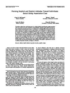
kernels, (2) explicit computation is promising for graphs with a uniform label structure, which exhibit few different features, and then scales to larger data sets. Synthetic data sets: In order to systematically vary the label diversity we generated synthetic graphs by the following procedure: The number of vertices was determined by Poisson distribution with mean 20. Edges were inserted between a pair of vertices with probability 0.1. The label diversity depends on the parameter pV . Edges were uniformly labeled; a node obtained the label 0 with probability 1 − pV . Otherwise the labels 1 or 2 were assigned with equal probability. In addition, we vary the data set size N between 100 and 300 adding 20 randomly generated graphs in each step. We analyze the runtime to compute the N × N kernel matrix. For the product graph based computation κV and κE are Dirac kernels. The results are depicted in Fig. 1(a), were a label diversity of 50 means that pV = 0.5. The runtime for implicit computation increases with the data set size and decreases with the label diversity. This observation is in accordance with our hypotheses. When the label diversity increases, there are less compatible pairs of vertices and the product graph becomes smaller. Consequently, computation of the product graph and the counting of weighted walks require less runtime. For explicit computation we observe a different trend: While the runtime increases with the size of the data set, the approach is extremely efficient for graphs with uniform labels (pV = 0) and becomes slower when the label diversity increases. Both approaches yield the same runtime for a label diversity of pV ≈ 0.3, while for higher values of pV implicit computation is preferable and explicit otherwise. Molecular data sets: We use a data set of graphs derived from small molecules (NCI Open Database, GI50, U251; http://cactus.nci.nih.gov) to analyze the runtime on a realworld data set with fixed label diversity. Vertex labels correspond to the atom types and edge labels represent single, double, triple and aromatic bonds, respectively. This time we vary the walk length and the data set size. Figure 1(b) shows that the runtime of implicit computation heavily depends on the size of the data set. The increase with the walk length is less considerable. This can be explained by the time TW DPG required to compute the product graph that is always needed independent of the walk length. For short walks explicit computation is very efficient, even for larger data sets. However, when a certain walk length is reached the runtime increases drastically. This can be explained by the growing number of different label sequence. Notably for walks of length 8 and 9 the runtime increases significantly with the data set size. This indicates that the time Tdot has a considerable influence on the runtime. For walk length up to 7 explicit computation beats implicit computation on the molecular data set. Weisfeiler-Lehman label refinement: Walk kernels have been successfully combined with label refinement techniques [7]. Weisfeiler-Lehman label refinement (WL) was proposed as a heuristic for the graph isomorphism problem, but has recently been applied to develop graph kernels [12].
Fig. 1. Runtime to generate kernel matrix by implicit and explicit computation of walk kernels.
To further analyze the sensitivity w.r.t. label diversity, we use the Enzyme data set [8], which consists of graphs with three initial node labels, with 0 to 3 iterations of WL, see Fig. 1(c). If no refinement is applied, the explicit mapping approach beats the product graph based algorithm for the used walk lengths. However, as soon as a single iteration of label refinement is performed, the product graph based algorithm becomes competitive for walk length 0 and 1 and outperforms the explicit mapping approach for higher walk lengths. The runtimes do not change significantly for more iterations of refinement. This indicates that a single iteration of WL results in a high label diversity that does not increase significantly for more iterations on the Enzyme data set. When using our walk-based kernel as base kernel of a WL graph kernel [12], our observation suggests to start with explicit computation and switch to implicit after few iterations of refinement. VIII. C ONCLUSION The breadth of problems requiring to deal with graph data is growing rapidly and graph kernels have become an efficient and widely-used method for measuring similarity between graphs. Highly scalable graph kernels have recently been proposed for graphs with thousands and millions of nodes, both for graphs with and without node attributes, based on explicit graph feature maps. These recent successes suggests that there is no benefit of the kernel trick – computing feature maps implicitly – when it comes to graphs. In this paper, we have empirically shown that this is not the case. In contrast, already for rather small walk lengths, implicit kernel computation is considerably faster than explicit computation. To set the stage for the experimental comparison, we actually made several contributions to the theory and algorithmic of graph kernels. We presented a first step towards a unified view on implicit and explicit graph features. More precisely, we gave a sufficient condition for when an explicit mapping from the implicit feature space of convolution kernels to a vector-valued feature space is possible. Using this results, we developed explicit computation schemes for random walk kernels [2], [3], subgraph matching kernels [2], [4], and shortest-path kernels [5]. This finally set the stage for our experimental comparison and its main result, a computational phase transition for walk kernels.
For future work, one should develop explicit computation schemes for other implicit graph kernels and vice versa. ACKNOWLEDGMENT This work grew out of discussions within the DFG Collaborative Research Center SFB 876. R EFERENCES [1] D. Haussler, “Convolution kernels on discrete structures,” University of California, Santa Cruz, CA, USA, Tech. Rep. UCSC-CRL-99-10, 1999. [2] T. G¨artner, P. Flach, and S. Wrobel, “On graph kernels: Hardness results and efficient alternatives,” in Learning Theory and Kernel Machines, ser. Lecture Notes in Computer Science, B. Sch¨olkopf and M. Warmuth, Eds. Springer Berlin / Heidelberg, 2003, vol. 2777, pp. 129–143. [3] S. V. N. Vishwanathan, N. N. Schraudolph, R. I. Kondor, and K. M. Borgwardt, “Graph kernels,” JMLR, vol. 11, pp. 1201–1242, 2010. [4] N. Kriege and P. Mutzel, “Subgraph matching kernels for attributed graphs,” in Int. Conf. on Machine Learning (ICML), 2012. [5] K. Borgwardt and H.-P. Kriegel, “Shortest-path kernels on graphs,” in Int. Conf. on Data Mining (ICDM), 2005, pp. 74–81. [6] H. Kashima, K. Tsuda, and A. Inokuchi, “Marginalized kernels between labeled graphs,” in Int. Conf. on Machine Learning (ICML), 2003. [7] P. Mah´e, N. Ueda, T. Akutsu, J.-L. Perret, and J.-P. Vert, “Extensions of marginalized graph kernels,” in Int. Conf. on Machine Learning (ICML), 2004. [8] K. M. Borgwardt, C. S. Ong, S. Sch¨onauer, S. V. N. Vishwanathan, A. J. Smola, and H.-P. Kriegel, “Protein function prediction via graph kernels.” Bioinformatics, vol. 21 Suppl 1, pp. i47–i56, 2005. [9] Z. Harchaoui and F. Bach, “Image classification with segmentation graph kernels,” in IEEE Conference on Computer Vision and Pattern Recognition (CVPR), 2007, pp. 1–8. [10] N. Shervashidze, S. Vishwanathan, T. Petri, K. Mehlhorn, and K. Borgwardt, “Efficient graphlet kernels for large graph comparison,” Journal of Machine Learning Research - Proceedings, vol. 5, pp. 488–495, 2009. [11] T. Horv´ath, T. G¨artner, and S. Wrobel, “Cyclic pattern kernels for predictive graph mining,” in Proceedings of Knowledge Discovery in Databases (KDD), 2004, pp. 158–167. [12] N. Shervashidze, P. Schweitzer, E. van Leeuwen, K. Mehlhorn, and K. Borgwardt, “Weisfeiler-lehman graph kernels,” JMLR, vol. 12, pp. 2539–2561, 2011. [13] J. Ramon and T. G¨artner, “Expressivity versus efficiency of graph kernels,” in First International Workshop on Mining Graphs, Trees and Sequences, 2003. [14] M. Neumann, N. Patricia, R. Garnett, and K. Kersting, “Efficient graph kernels by randomization,” in Machine Learning and Knowledge Discovery in Databases (ECML/PKDD), 2012, pp. 378–393, long version arXiv:1410.3314 [stat.ML]. [15] A. Feragen, N. Kasenburg, J. Petersen, M. de Bruijne, and K. Borgwardt, “Scalable kernels for graphs with continuous attributes,” in Advances in Neural Information Processing Systems 26. Curran Associates, Inc., 2013, pp. 216–224. [16] N. Wale, I. A. Watson, and G. Karypis, “Comparison of descriptor spaces for chemical compound retrieval and classification,” Knowl. Inf. Syst., vol. 14, no. 3, pp. 347–375, 2008.