In this paper our existing Bayesian method for defining and using a very flexible
class of prior ... specifically to classification and regression tree (C&RT) models.
Following [1], we ..... for Nonlinear Classification and Regression. Wiley (2002). 2.
Exploiting Informative Priors for Bayesian Classification and Regression Trees Nicos Angelopoulos and James Cussens Department of Computer Science University of York Heslington, York YO10 5DD, UK {nicos|jc}@cs.york.ac.uk
Abstract. A general method for defining informative priors on statistical models is presented and applied specifically to the space of classification and regression trees. A Bayesian approach to learning such models from data is taken, with the Metropolis-Hastings algorithm being used to sample from the posterior. By only using proposal distributions closely tied to the prior, acceptance probabilities are determined by likelihood ratios alone, whatever the prior used. Our approach is empirically tested by varying (i) the data, (ii) the prior and (iii) the proposal distribution. A comparison with related work is given.
1
Introduction
A key feature of the Bayesian approach to statistical inference is that prior knowledge (i.e. information available prior to data) can be incorporated into the learning process in a mathematically rigorous and conceptually clear manner. On the assumption that a space of possible statistical models can be defined, prior knowledge is expressed via a prior distribution over this space. This distribution is then updated with the data using Bayes theorem to produce a posterior distribution. The Bayesian framework is compellingly simple, but there are many complexities in applying it to real data analysis. Many of these difficulties are computational. For example, in high-dimensional spaces the posterior will be too complex to report directly so features of the distribution (typically the mean and variance) must be extracted—requiring, in general, a difficult integration. These problems are being progressively alleviated by increased computing power and the subsequent use of Markov chain Monte Carlo (MCMC) techniques to sample from the posterior. In this paper our existing Bayesian method for defining and using a very flexible class of prior distributions over models is further developed and applied specifically to classification and regression tree (C&RT) models. Following [1], we use C&RT rather than CART as an abbreviation, since the latter is a registered trademark of California Statistical Software, Inc. C&RT models [2] are so well known in machine learning (and increasingly statistics) that this paper assumes familiarity with the basic properties of these models.
The method is fully Bayesian using a version of the Metropolis-Hastings MCMC algorithm which can sample from posterior distributions over the space of all possible C&RT models. Even after eliminating a priori uninteresting trees (for example, those containing sparsely populated leaves) this will be a very large space. The key feature of our approach is that the user can apply whatever prior knowledge s/he has available to restrict and/or bias the prior distribution over this space. Also, in contrast with other Bayesian C&RT work, MCMC sampling from the space is almost entirely driven by sampling from the prior. The rest of the paper is structured as follows. Section 2 describes our language for defining priors. Section 3 describes the specific priors that have been used for Bayesian inference of C&RT models. Section 4 presents our version of the Metropolis-Hastings (MH) algorithm and gives some convergence properties for an important special case. Section 5 describes the various experiments we set up to test our method and Section 6 gives a representative sample of the results of those experiments. The paper concludes with a comparison with related work (Section 7) followed by conclusions and pointers to future work (Section 8).
2
Defining priors with stochastic logic programs
Our approach to defining priors is related to a line of research which was independently initiated by [3] and [4]. The basic idea is to specify a prior distribution over a space of models with a stochastic program rather than by some closed-form expression: Instead of specifying a closed-form expression for the tree prior, p(T ), we specify p(T ) implicitly by a tree-generating stochastic process. Each realization of such a process can simply be considered a random draw from this prior. [3] A particularly convenient language for defining such stochastic programs is stochastic logic programming [5]. A stochastic logic program (SLP) can be used to define a prior over a given space of statistical models by a two-step process. Firstly, a standard logic program is written which defines the desired model space (the hypothesis space in machine learning parlance). We simply define a unary predicate cart/1 in a logic program such that each instantiation for X which makes cart(X) true is a term in first-order logic which represents a C&RT model in the hypothesis space. We can exploit the expressiveness of first-order logic to represent C&RT models, choosing the most convenient logical representation. At this point any C&RT models we wish to exclude from the hypothesis space can be so excluded by adding the appropriate constraints to the logic program. For example, the logic program in Table 1 defines the space of binarysplitting C&RT models where there are only three binary attributes x1 , x2 and x3 . Since the xi are binary it suffices to supply the variable to determine the splitting rule—assume that data for which xi = 0 go down the left branch and data for which xi = 1 go down the right branch. To restrict, for example, the hypothesis space to have only trees where x1 is the top node it is enough to
define cart_foo(X) :- X = x1-[L,R], cart(X). and use cart foo/1 as the predicate defining the hypothesis space. cart(leaf). cart(Split-[L,R]) :- choose_split(Split), cart(L), cart(R). choose_split(x1).
choose_split(x2).
choose_split(x3).
Table 1. A logic program defining a space of C&RT models
The second step of defining the stochastic element of the SLP is most easily understood by first considering how the logic programming language Prolog searches for logical consequences of a logic program. Given a query such as :cart(X). (“find X such that cart(X) is true”), Prolog will search for suitable Xs with a deterministic depth-first search. When there is a choice of rules each of which might lead to a proof, Prolog always chooses whichever rule occurs first in the logic program. If this rule leads to a dead-end, then Prolog backtracks and tries the second rule, and so on. The basic SLP idea is simple: probability labels are attached to rules in the logic program thus converting it into an SLP. Now when the search for proofs has to choose between rules, a rule is chosen probabilistically according to the probability labels. In this paper, if a chosen rule does not lead to a proof, then backtracking will try from amongst untried rules, renormalising the probabilities as necessary. This approach to backtracking is backtrackable sampling [6] and is, by far, the most efficient SLP sampling mechanism. Now when the query :- cart(X). is asked, there is a distribution over possible instantiations for X. Since each X represents a C&RT model, this provides a prior distribution over this model space. In this paper we have extended the representational power of SLPs so that probability labels may be computed ‘on the fly’ rather than being fixed. For example, Table 2 shows an SLP based on Table 1 where the probability of growing a tree by splitting a leaf depends on the depth of that leaf. Table 2 uses a simplified version of our syntax adopted for the purposes of introducing our SLPs. 1 - 1/D : cart(leaf). 1/D : cart(Split-[L,R]) :- NewD is D+1, choose_split(Split), NewD:cart(L), NewD:cart(R). choose_split(x1).
choose_split(x2). choose_split(x3).
Table 2. Prior distribution over C&RT models where the probability of splitting a leaf depends on the depth of the leaf, where D > 0.
3
Priors for Bayesian C&RT
In this section we describe the actual priors we have used for the experiments described in Section 5. Since this paper’s purpose is to report on the strengths and weaknesses of our method, rather than analyse a particular dataset, we focus on general issues concerning the definition of priors, rather than tailoring a prior to reflect some actual domain knowledge. Fixing some notation, note that a given C&RT model T maps an example described by a set of p predictor variables X = X1 , X2 , . . . Xp to a distribution over a response variable Y . In the case of classification trees (also known as decision trees) Y is discrete and finite, and in the case of regression trees Y is continuous. Some C&RT implementations throw away information given by the distribution of Y and simply return the majority class or mean value as appropriate, but this is just a design decision. Fundamentally it is a distribution over Y that is given. It follows that each tree T defines a conditional probability distribution P (Y |T, X). For the purposes of determining a posterior distribution over trees, this conditional distribution is a likelihood function as the following version of Bayes theorem indicates: P (T |Y, X) =
P (T |X)P (Y |T, X) P (Y |X)
The key point is that the prior P (T |X) is conditional on the predictor variables, i.e. we can use the observed values of X in the data to help define sensible priors. Importantly, this allows us to rule out a priori trees with leaves which contain few examples. Although it is conceivable that acceptable trees might have sparsely populated leaves (since if further data were collected they might no longer be empty) ruling out such trees is normal in this research area and greatly reduces the size of the model space. In our experiments only trees whose leaves have at least 5 examples are permitted, following [4]. Clearly, this value can be altered: for example, the rpart tree-building package in the R statistical system uses a default value of 20. The predictors X could also be used to define a prior biassed towards even splits of the data if so desired, but we have yet to investigate the desirability of such an option. In this paper we use two types of priors over trees. The first type, the GROWTREE prior, is essentially that used by [3]. The stochastic process which defines a GROWTREE prior grows a C&RT tree by starting with a single leaf node and then repeatedly splits each leaf node η with a probability α(1 + dη )−β , where dη is the depth of node η and α and β are prior parameters set by the user to control the size of trees. Unsplit nodes become leaves of the tree. If a node is split, the splitting rule for that split is chosen uniformly. An abbreviated fragment of the SLP which expresses this prior is given in Table 3. The other type of prior is the EDITTREE prior. Here an ‘initial’ C&RT model is supplied. This can be any tree, for example the tree produced by the standard greedy algorithm or one manually entered by the user. This tree is
%split_cart(Tree,Alpha/Beta parameters) split_cart([H|T],Alpha/Beta) :- ... Split is Alpha*exp((1+D),-Beta), %split prob [Split]:split_leaf(D,Ids,P,LV,RmLvPrs,NxLvPrs), split_cart(NxLvPrs,Alpha/Beta). split_cart([],_ABeta ). Split:Split::split_leaf(D,Ids,[Hp|Tps],LV,LvPrs,NwLvPrs) :D1 is D + 1, ... %increase depth branch(Rest,ChL,PL), branch(Rest,ChR,PR), ... (1 - Split):Split::split_leaf(D,Ids,P,leaf(D,Ids,P),LvPrs,LvPrs). Table 3. GROWTREE prior fragment defined with an SLP
then probabilistically edited. This approach is closely related to the proposal mechanisms of [3, 4, 1]. Hopefully, the EDITTREE SLP fragment in Table 4 conveys the general idea. With probability 4/5 the tree is edited. There are three possible editions: growing the tree by splitting a leaf, pruning the tree by merging neighbouring leaves and changing a splitting rule. These are chosen with equal probability. In a sense, the GROWTREE prior is a special case of EDITTREE where the empty tree is edited and may only be edited by being grown. 4/5 :: edit(CartIn,CartOut) :- one_edit(CartIn,CartMid), edit(CartMid,CartOut). 1/5 :: edit(CartIn,CartOut) :- one_edit(CartIn,CartEdt), edcart_to_concrete_cart(CartEdt,CartOut). 1/3 :: one_edit( CartIn, CartOut ) :- ... % grow by splitting a leaf 1/3 :: one_edit( CartIn, CartOut ) :- ... % prune by merging neighbours 1/3 :: one_edit( CartIn, CartOut ) :- ... % change a splitting rule Table 4. EDITTREE prior defined with an SLP
4
Using the Metropolis-Hastings algorithm
Recall that the Metropolis-Hastings (MH) algorithm is an MCMC algorithm which defines a Markov chain (T (i) ) with a transition kernel K(ti , ti+1 ) as follows. If T (i) = t(i) , then T (i+1) is produced by generating Ti0 ∼ q(t0 |t(i) ) for some proposal distribution q. An acceptance probability α(t, t0 ) is used to decide whether to accept the proposed t0 . t(i+1) = t0 with probability α(t, t0 ) (the proposed t0 is accepted) and t(i+1) = t(i) with probability 1 − α(t, t0 ). By setting
the acceptance probability like this: �
0
α(t, t ) = min
� P (t0 |x, y) q(t|t0 ) ,1 P (t|x, y) q(t0 |t)
(1)
the chain (T (i) ) will converge to sampling from the desired posterior P (T |X = x, Y = y) under weak conditions. It is not difficult to see (via Bayes theorem) that if q(t|t0 )P (t0 ) = q(t0 |t)P (t) i.e. q satisfies the detailed balance condition with the prior P as an invariant distribution for q, then: � � P (y|t0 , x) 0 ,1 (2) α(t, t ) = min P (y|t, x) In our approach we always choose proposal distributions q which permit this simplification of the acceptance probability. The crucial point is this: such a choice of q ensures that α(t, t0 ) is always determined by the simple likelihood ratio in (2), no matter how complex the prior is. Without this assurance, the combination of a flexible logic-based representation and efficient (backtrackable) 0 0 |x)P (y|t0 ,x) |x,y) in (1) equals PP(t(t|x)P sampling would be unusable. The ratio PP(t(t|x,y) (y|t,x) but computing the prior probability P (t|x) for any given C&RT model t (as opposed to merely sampling from the prior) would be prohibitively expensive. This contrasts with [3] where “specifications [which] allow for straightforward evaluation of p(T ) for any T ” are required. Since our trees do not explicitly define a distribution over classes at the leaves of the tree, our likelihoods are marginal likelihoods—we integrate over all possible class distributions. To do this, we use exactly the same approach as [3, 4, 1]. For each leaf, the uniform Dirichlet distribution (all parameters set to 1) is the distribution over all possible distributions over classes. The Dirichlet assumption allows a closed from for the marginal likelihood P (Y |X, T ). Since we can readily sample from any of our priors (as described in Section 2) one simple choice for the proposal is to set q(t0 |t) = P (t0 ): a version of the independent MH algorithm [7, p. 239]. In this case, trivially q(t|t0 )P (t0 ) = q(t0 |t)P (t). There are a number of known useful results for this algorithm. Here is a result from [8] cited in [7] specialised to the current case: Theorem 1. If q(t0 |t) = P (t), then a uniformly ergodic chain is produced by the independent MH algorithm if there exists a constant M such that P (t|x, y) ≤ M P (t|x),
t ∈ supp P (·|x)
In this case, n
0
0
||K (t, t ) − P (t |x, y)||TV
�
1 ≤2 1− M
�n (3)
where || · ||TV denotes total variation norm. The constant M always exists as long as the observed data y has positive prior probability/density (an implicit assumption in all Bayesian approaches).
The bound (3) shows that the Markov chain produced by sampling from the prior and accepting moves using (2) has a rate of convergence to the posterior which is faster the closer the prior is to the posterior. Unfortunately, unless the prior happens to be a good approximation of the posterior, there is no reason to expect M to be small enough for fast convergence—indeed the results reported in Section 6 indicate unacceptably slow convergence with proposals of this type. The basic problem with proposing new trees using the prior is that only non-local moves in the space of trees are proposed. Once the chain has found a tree with high likelihood then new trees proposed via the prior are very unlikely to be accepted, and the chain gets stuck. Once a high likelihood tree has been found it is better to ‘explore its neighbourhood’ in the hope of finding similarly high likelihood trees. Fortunately a neighbourhood structure is built into the SLP approach. Suppose a tree t has been sampled from the prior. The stochastic process which led to t being output involved a sequence of probabilistic choices where rules were selected according to the probability labels attached to them. To sample a tree t0 in the immediate neighbourhood of t it is enough to force the process to backtrack to the last available choice-point and then to run the stochastic process forwards from that point in the normal manner. Bigger jumps are effected by first backtracking through several choice points and then sampling ‘forward’. (Of course, sometimes we may end up with t0 = t but usually a new tree is proposed.) Sampling from the prior is just a special case of this approach where backtracking is constrained to always take the process back to the very first choice point. Let qk denote a proposal distribution which backtracks until it is k choice points from the initial choice point, so that q0 denotes the independent MH algorithm. If k is too big for the number of choice points available then qk just proposes the current model. Note that the degree of backtracking is entirely deterministic, in contrast to a related approach in [9]. This ensures that detailed balance holds. Although detailed balance holds and thus (2) can be used to compute the acceptance probability for qk , qk will not produce an irreducible chain unless k = 0, which is the independent MH algorithm. Just doing local proposals restricts the chain to exploring only part of the space, and so it is necessary to select k = 0 with positive probability so that the initial choice point is sometimes reached, thus effecting arbitrarily big (‘global’) proposals. In our experiments we have tried a number of ways of combining qk kernels for varying values of k. As we see in the next section using local jumps gives better convergence than the independent MH algorithm.
5
Experimental set-up
In our experiments we have used two datasets: the Wisconsin breast cancer data (BCW) and the Kyphosis dataset (K). BCW was originally donated to the UCI depository by Wolberg [10] and was used by [3]. Dataset K comes as part of
the rpart R package for building and manipulating classification and regression trees. BCW contains 16 missing data values. Following [3] we have simply deleted datapoints which contain missing values. In both cases the machine learning task is binary classification using integer-valued predictors—nine predictors in the case of BCW, and three for K. All splits are binary: made by splitting on some threshold. There are 683 datapoints for BCW and 81 for K. We have used the GROWTREE prior with α = 0.95 and with β taking values 0.5, 1 and 1.5 to give a bias towards big, medium and small trees respectively. For our experiments with the BCW data, we also used two versions of the EDITTREE prior—one with a greater bias towards editing than the other. In both cases the initial tree from which editing begins is that of [3, Fig 1]. We have experimented with a number of ways of combining local and global proposals. We have some results using q0 which is simply the independent MH algorithm where all proposals are global. We will denote q0 by ND0 for a uniform nomenclature. We also have two variants using qk where in one k cycles through the values 0, 1, 2, . . . 7 (ND7) and in the other k cycles through the values 0, 1, 2, . . . 50 (ND50). A final variant (RN) randomly chooses a value of k so that a choice point to backtrack to is chosen uniformly from all those to which backtracking is possible. If, as is common, there are many available points this means that RN will rarely backtrack to choice points near the initial choice point, so RN is heavily biassed against global proposals. To enable a comparison with [9] we have also used the proposal mechanism (FD), which has a more complex expression for the acceptance probability.
6
Experimental results
We have performed a large number of experiments, and analysed the results in many ways. Generally speaking the results are as expected: the method works but more work needs to be done in ensuring rapid convergence of the chain to the posterior. We used Sicstus Prolog 3.11 running under Linux on two machines each with a 2.4GHz processor and at least 512Mb RAM. The computation of the log-likelihood ratio uses a C function called from Prolog. Running a chain for 60,000 iterations typically took 1-2 hours but with the quickest chain taking 30 minutes and the slowest 6 hours. This variation in speed is determined by the average size of the C&RT model and by the backtrack strategy. The following sections aim to summarise our results by focusing on some of the more important issues. Throughout we use graphs of log-likelihood mapped against the iteration number of our MCMC algorithm (log-likelihood trajectories), since we have found this gives the best insight into the behaviour of the chain. We have not used a ‘burn-in’ to throw away initial iterations since we actually want to see how quickly the chain moves into an area of reasonably high log-likelihood.
6.1
Comparison to the standard C&RT algorithm
The contrasts between Bayesian C&RT and the standard greedy algorithm for building a single C&RT model have been well explored in the existing Bayesian C&RT literature [3, 4, 1]. The basic point is that the Bayesian method represents posterior uncertainty better and makes a more thorough exploration of the model space. This is at the cost of more computation. Interestingly, the Bayesian aspect of Bayesian C&RT can be ignored and the MCMC approach be seen simply as a stochastic search for small trees which fit the data well; which is the basic goal of the standard greedy approach. Unsurprisingly the greater degree of search in our approach allows greater success in meeting this goal. The rpart (recursive partitioning) R package implements a version of the standard greedy algorithm. By default, 10-fold cross-validation is used to prune trees to avoid overfitting. The trees found by rpart for datasets BCW and K using default settings have log-likelihoods (i.e. fit to data) -97 and -39, and sizes 7 and 5, respectively. (Throughout we round log-likelihoods to the nearest integer.) By looking through the log of visited trees it is easy to find ‘better’ trees for many of the combinations of prior and MH variant that we use. For BCW we can find a tree with only 5 leaves and log-likelihood of -86 and for K a tree with only 3 leaves and log-likelihood of -36. 6.2
Analysing convergence
Fig 1 records the trajectories of the log-likelihood as the MH algorithm moves through the space of trees. In both cases exactly the same experimental parameters have been used, just the random seed has been altered. We can see that although the distribution of log-likelihoods is similar in both cases, it appears that the two chains have wandered into different areas of tree space: the righthand trajectory has more plateaux and also reaches higher log-likelihoods than the lefthand one. 6.3
Using local jumps
Local jumping helps prevent getting stuck. The log-likelihood trajectory using ND7 shown in Fig 2, shows that the big jumps which ND7 proposes are rarely accepted, so the chain remains stuck at the same model for long periods. This problem is even more pronounced if ND0, the independent MH algorithm,is used. Compare this with Fig 1, where RN is being used. On the other hand, FD gave similar results to RN. 6.4
Influence of a strong prior
Fig 3 compares log-likelihood trajectories using the EDITTREE prior and the GROWTREE prior respectively with all other parameters being equal. The distinct horizontal line in the EDITTREE trajectory is clear evidence that the EDITTREE prior is pulling the Markov chain back to the initial tree. Note that Figs 2-3 all contain initial very low log-likelihoods which are invisible on the graphs.
-75
-75
’tr_rn1_a0_95b1_bcw_data_i60K__s1__scaled.llhoods’
-80
-80
-85
-85
-90
-90
-95
-95
-100
0
10000
20000
30000
40000
50000
60000
-100
’tr_rn1_a0_95b1_bcw_data_i60K__s3__scaled.llhoods’
0
10000
20000
30000
40000
50000
60000
Fig. 1. Log-likelihood trajectories using two different seeds (low values truncated). Prior=GROWTREE (β = 1), Data=BCW, MCMC=RN -50
’tr_nd7_a0_95b1_bcw_data_i60K__s1.llhoods’
-100
-150
-200
-250
-300
0
10000
20000
30000
40000
50000
Fig. 2. Log-likelihood trajectory. Prior=GROWTREE (β MCMC=ND7
7
60000
=
1), Data=BCW,
Comparison with related work
This paper lies at the intersection of two lines of work: that on Bayesian C&RT [3, 4, 1] and that on using SLPs for general Bayesian model inference [6, 9]. The SLP work had claimed to provide a general Bayesian machine learning method but had only results for model spaces composed of Bayesian nets. This paper backs up this initial claim by applying the basic framework of [9] to C&RT model space. The SLP method has also been improved in a number of ways: (i) probabilities no longer need be hard-coded constants, (ii) the use of backtracking adds an element of search to the probabilistic sampling—greatly increasing the efficiency of the sampling and (iii) the proposal mechanism can now use deterministic backtracking thus permitting a simple form (2) for the acceptance probability. The most obvious difference from the Bayesian C&RT work is that here all (non-parameter) priors are defined by an SLP. However, SLPs can encode priors
-60
-50
’tr_rn1_a0_95b1_edit_data_i60K__s9.llhoods’
’tr_rn1_a0_95b1_bcw_data_i60K__s1.llhoods’
-65 -100 -70
-75
-150
-80 -200
-85
-90 -250 -95
-100
0
10000
20000
30000
40000
50000
60000
-300
0
10000
20000
30000
40000
50000
60000
Fig. 3. Log-likelihood trajectories. In both cases: Data=BCW, MCMC=RN. For LHS: Prior=EDITTREE. For RHS: Prior=GROWTREE (β = 1)
originally expressed in other formalisms: in Section 3 the GROWTREE prior was written to encode (essentially) the prior given in [3]. Secondly, here there is only one way of proposing new C&RT models; by backtracking and then forward sampling using the prior. In the other Bayesian C&RT work a variety of moves are used—five are listed in [1, p. 161]. This restriction is a disadvantage of our approach, since it compels the user to ensure that the SLP used to express the prior encodes an appropriate neighbourhood structure (models with similar likelihood should be mutually reachable by shallow backtracking). The consequent advantage is that such a restriction ensures that no prior terms complicate the acceptance probability. Constraining the proposal mechanism to produce such an acceptance probability is also a choice taken in [1]—although for this to work the proposal mechanism has to depend upon global parameters of the current tree. The biggest contrast with previous Bayesian C&RT work is that we permit big jumps by choosing small values of k for our proposal distribution qk . In [1] it is noted that pruning off any given branch of a tree is straightforward in their approach but that how to generate a similar branch (to maintain reversibility) “is not obvious”. In the approach presented here it is obvious, we just sample forward from the relevant choice point. In [1] also noted is the danger that many big jumps will propose trees with sparsely populated leaves—we avoid this problem by simply compelling the proposal mechanism to search for trees with adequately populated leaves. Of course, this element of search slows down the speed with which proposals are made, but this appears to be compensated for by only having interesting candidate models proposed.
8
Conclusions and future work
We have a working system (http://www.cs.york.ac.uk/~nicos/sware/slps) which permits the user to express prior information about model structure by writing an SLP. So far, the software has been applied to graphical models (e.g.
Bayesian nets) and C&RT models. The comparison of GROWTREE and EDITTREE results show that prior information has the desired effect of significantly altering the posterior (at least for the moderately sized datasets used here). However, the current system has a number of shortcomings. Despite the encouraging theoretical result in Section 4 on convergence of the independent MH algorithm (here denoted by q0 as well as by ND0) all our results, not just those presented, indicate that local jumps are essential to adequately explore the posterior. The next crucial bit of theoretical work is to extend Theorem 1 to apply to transition kernels involving qk where k > 0. This will guide the choice of transition kernel in contrast to our current empirical approach. At present, it appears that our proposals which permit local jumps (e.g. RN as used for Fig 1) are too heavily biassed towards local jumps leading to the chain getting stuck in local areas of tree space. Concerning actual implementation of the chain, our current program does not use Prolog’s built-in backtracking: if this were possible this would permit a significant speed-up. A more radical approach is to adapt an existing Prolog system to have our probabilistic mechanisms built-in. The nature of the MH algorithm also means that tabling could be used advantageously.
References 1. Denison, D.G.T., Holmes, C.C., Mallick, B.K., Smith, A.F.M.: Bayesian Methods for Nonlinear Classification and Regression. Wiley (2002) 2. Breiman, L., Friedman, J.H., Olshen, R.A., Stone, C.J.: Classification and Regression Trees. Chapman & Hall, New York (1984) 3. Chipman, H.A., George, E.I., McCulloch, R.E.: Bayesian CART model search. Journal of the American Statistical Association 39 (1998) 935–960 4. Denison, D.G.T., Mallick, B.K., Smith, A.F.M.: A Bayesian CART algorithm. Biometrika 85 (1998) 363–377 5. Muggleton, S.: Stochastic logic programs. In De Raedt, L., ed.: Advances in Inductive Logic Programming. IOS Press, Amsterdam (1996) 254–264 6. Cussens, J.: Stochastic logic programs: Sampling, inference and applications. In: Proc. UAI-00, San Francisco, CA, Morgan Kaufmann (2000) 115–122 7. Robert, C.P., Casella, G.: Monte Carlo Statistical Methods. Springer, New York (1999) 8. Mengersen, K.L., Tweedie, R.L.: Rates of convergence of the Hastings and Metropolis algorithms. Annals of Statistics 24 (1996) 101–121 9. Angelopoulos, N., Cussens, J.: Markov chain Monte Carlo using tree-based priors on model structure. In Breese, J., Koller, D., eds.: Proc. UAI-01, Seattle, Morgan Kaufmann (2001) 10. Wolberg, W.H., Mangasarian, O.L.: Multisurface method of pattern separation for medical diagnosis applied to breast cytology. Proceedings of the National Academy of Science 87 (1990) 9193–9196