Exploiting Parallelism in Automatic Di erentiation - Semantic Scholar

Exploiting Parallelism in Automatic Dierentiation Christian Bischof Andreas Griewank David Juedes

Mathematics and Computer Science Division Argonne National Laboratory Argonne, Illinois 60439-4801

Argonne Preprint MCS-P204-0191 Published in Proc. 1991 Int. Conf. on Supercomputing, E. Houstis and Y. Muraoka, Eds., ACM Press, Baltimore, Md., pp. 146-153, 1991.

Abstract. The numerical methods employed in the solution

of many scienti c computing problems require the computation of rst- or second-order derivatives of a function f : Rn ! Rm . We present an approach that, given a serial C program for the computationof f (x), derives a parallel execution schedule for the computation of f and its derivatives in a completely automatic fashion. This is achieved by overloading the computation of f (x) in C++ to obtain a trace of the computations to be performed and then transforming this trace into a data ow graph for the computation of f (x). In addition to the computation of f (x), this graph also allows us to exactly and inexpensively compute derivates of f by the repeated use of the chain rule. Parallelism is exploited in two ways: rows or columns of derivative matrices can be computed by independent passes through the computational graph, and parallelism within the processing of this computational graph can be exploited by processing independent subgraphs concurrently. We present experimental results that show that good performance on shared-memory machines can be obtained by using a graph interpreter approach. We then present some ideas that are currently under development for improving computational granularity and for implementing parallelautomaticdierentiationschemes in a portableand more ecient fashion.

1 Introduction The methods employed for the solution of many scienti c computing problems require the evaluation of derivates of some objective function. Probably best known are gradient methods for optimization and Newton's method for the solution of nonlinear systems [8, 10]. Other examples can be found in [9]. For example,  This work was supported by the Applied Mathematical Sciences subprogramof the Oce of Energy Research, U. S. Department of Energy, under Contract W-31-109-Eng-38. The third author was also supported through NSF Cooperative Agreement No. CCR-8809615.

given a function

f : Rn ! R; one can nd a minimizer x of f using variable metric methods that involve the iteration for i = 1, 2, .... do Solve Bi si = ?rf(xi ) xi+1 = xi + isi

end for

for suitable step multipliers i > 0. Here

0 rf(x) = B @

@ @x1 f(x)

.. . @ f(x) @x

1 CA

(1)

n

is the gradient of f at a particular point xo , and B is a positive de nite matrix that may change from iteration to iteration. For nding the root of a nonlinear function 0f 1 1 . . F : R n ! Rn ; F = B @ . CA ; fn Newton's method requires the computation of the socalled Jacobian matrix 0 @ f (x)


@ f (x) 1 @x1 1 @x 1


A : (2) F 0(x) = @


@ fn (x)


@ fn (x) @x1 @x n

n

Then we execute the following iteration: for i = 1, 2, .... do Solve F 0(xi )si = ?F(xi) xi+1 = xi + si

end for

In many applications, F 0 is large and sparse, and the solution of an equation system involving F 0 requires the use of an orthogonal factorization. From the viewpoint of the designers of mathematical software, the computation of derivatives was often considered to be expensive. If derivative information was employed, derivatives were approximated by nite dierences, or the user was required to provide a program that computed the necessary derivative information. Both alternatives are unsatisfactory, as nite dierence approximations can lead to loss of accuracy, and the computation of derivatives by hand is tedious and error-prone. One has to keep in mind that, in particular for largescale problems, the objective function usually is not represented in closed form, but is given in the form of a computer program that computes f or an approximation thereof. Symbolic dierentiation techniques currently are often not feasible, since they do not fully

utilize common subexpressions, and therefore are computationally inecient. These issues are discussed in more detail in [12]. The situation is even more complicated if one wishes to exploit parallelism. Considerable progress has been made in the implementation of linear algebra kernels, such as orthogonal factorizations, on parallel machines [2, 3, 21, 23]. With respect to the computation of derivative information, approaches to computing nitedierence approximations in parallel using graph coloring approaches have been successful [7, 19, 22], but again accuracy may be lost. We, in turn, suggest the use of automatic dierentiation to compute derivative information. This approach computes derivative information without truncation error, and in an automatic fashion. That is, a user can take a black-box view of the dierentiation process. Automatic dierentiation techniques rely on the fact that every function, no matter how complicated, is executed on a computer as a (potentially very long) sequence of elementary operations such as additions, multiplications, and elementary functions such as sin and cos. By applying the chain rule @ @ @ @t f(g(t))jt=t ) = ( @s f(s)js=g(t ) )( @t g(t)jt=t ) (3) over and over again to the composition of those elementary operations, one can compute derivate information of f exactly and in a completely mechanical fashion. In the next section, we will expand on the ideas behind automatic dierentiaton and give an overview of the various ways in which it can be implemented. In section 3, we then discuss how automatic dierentiation can be used to derive in an automatic fashion a parallel execution schedule for the computation of the objective functions and its derivatives. We also present some experimental results obtained on the Symmetry. In Section 4 we discuss ongoing work to improve the eciency of parallel automatic dierentation. o

o

if ((x1 - 2) > 0) then a = x1

else

a = 2*x1

end if

b=1 for i = 1:2 do b = b + sqrt(b)*a

end for

y0 = b/x2 y1 = a*x2

Figure 1: Sample Program i 1: 2: 3: 4: 5: 6: 7: 8: 9: 10: 11: 12: 13:

o

operation

ti

di

di

x1 = 1 x2 = 1.5 r1 = x1 - 2 r1 = 2 * x1 r2 = 1 r3 = sqrt(r2) r4 = r1 * r3 r2 = r2 + r4 r3 = sqrt(r2) r4 = r1 * r3 r2 = r2 + r4 y1 = r2 / x2 y2 = r1 * x2

1 1.5 1 2 1 1 2 3 1.73 3.46 6.46 4.31 3

1 0

4.41 -2.87

2 0 0 2 2 0.58 4.61 6.62 4.41 3

2.21 1.05 2.10 1.05 1.05 1.33 0.67 0.67 1.0 0

?

?

Figure 2: Trace of Function Execution we change the initializations in line 1 and 2 accordingly. To compute derivatives in an automatic fashion, we now associate a unique variable ti , i = 1; 13 with each computed value. This value (rounded to three signi cant digits) is shown in the column labeled ti in Figure 2. Derivatives can now be computed by associating a value di with each intermediate quantity and by using elementary dierentiation arithmetic. For example, if we wish to compute @x@ 1 F(x1; x2)j(x1 ;x2 )=(1;1:5), @t for every intermediate quantity ti. di will hold @x 1 Hence, after setting d1 = 1 and d2 = 0, we can proceed to d12 = @x@ 1 f1(x1 ; x2)j(x1 ;x2)=(1;1:5) and d13 = @ @x1 f2(x1 ; x2)j(x1 ;x2)=(1;1:5) by simple use of the chain rule. For example, if tj = tk + tl ; then dj = dk + dl : For tj = tk  tl ;

2 Automatic Dierentiation The idea behind automatic dierentiation is best understood through an example. Assume that we have the sample program shown in Figure 2 for the computation of a function F : R2 ! R2. Here, x1 and x2 are the independent variables, and y1 and y2 the dependent variables. If we were to execute this program to compute F(1; 1:5), the the list of elementary instructions shown in Figure 2 would be executed. Here r1 through r4 refer to main memory or register locations where intermediate results are stored. The code shown in Figure 2 is a trace of the computations performed to compute F(1; 1:5). As long as x1 < 2, this trace can be used as a blueprint for the computation of F(x1; x2), when

i

2

we have

it can be shown that for an intermediate quantity tj whose value is used in the computation of tk ; k 2 Ij , we have X @gk  dj = dk k2I @xj where gk is the elementary operation that de nes tk . This is best understood with an example. Assume that we wish to compute rf1 (x1; x2)j(x1 ;x2 )=(1;1:5), that is, the rst row of the Jacobian of F. We then initialize d12 = 1 and d13 = 0. Since t2 alias x2 is used only in the computation of t12 and t13, we can compute @f1 = d = @g12  d + @g13  d : @x2 2 @t2 12 @t2 13 Now g12 = t11 =t2, and g13 = t4  t2 , so @g12 = ?t =(t )2 11 2 @t2 and @g13 = t : @t2 4 By starting from the dependent variables in this fashion, and traversing the computation in reverse order, we emerge at the independent variables with rf1. The adjoint quantities are shown in the column labeled i in Figure 2. If we were to compute rf2(x1 ; x2)j(x1 ;x2 )=(1;1:5), we could repeat this procedure with d12 initialized to 0 and d13 initialized to 1. Again we can compute all rows in one pass by associating an m-vector with each intermediate quantity, and a product wT J can be computed in one pass by initializing di = wi ; i = 1; : : :; n. Exploiting the sparsity of these vectors, one can bound the ratio between the cost of evaluating J rowwise and that of evaluating f by the maximum number of nonzeros in any column. Both the reverse and forward mode of automatic differentiation have been implemented in the ADOL-C package. Using the operator overloading features of C++, ADOL-C generates a computational trace (the so-called tape) of the evaluation of F(xo). First- and higher-order derivatives can then be computed using either the forward or reverse mode by passing over the tape in the appropriate fashion. While the tape itself may be quite large, it is always accessed in a purely sequential fashion, and RAM storage requirements are modest by exploiting the fact that only few temporary variables are active at any given point in time. Details can be found in [13]. We mention that the automatic dierentiation of computer arithmetic has been investigated since before 1960. Since then there have been various implementations of automatic dierentiation. Most of these implementations have concentrated on the simple forward evaluation of derivatives. For scalar functions of the form y = F(x1; :::xn), the forward evaluation of partial derivatives requires O(n) times the execution time

dj = t k  d l + t l  d k : For univariate functions g = g(t) such as sin, cos, or sqrt, tj = g(tk ) implies @ g(t )  d : dj = @t k k The values of the dj 's in our particular example are shown in the column labeled di in Figure 2. After we have traversed all statements, we have computed @ @x1 F(x1; x2)j(x1;x2 )=(1;1:5), i.e. the rst column of the Jacobian matrix. To obtain the second column of the Jacobian matrix, we initialize d1 = 0 and d2 = 1 and repeat the previous procedure. Since the propagation of the di's is about as costly as that of the ti 's, each derivative pass costs roughly the same as the evaluation of the original function. This mode of automatic dierentiation, where we

j

maintain the derivatives of intermediate quantities with respect to the independent variables, is called the forward mode of automatic dierentiation. Instead

of having two passes over the code, we could also have computed J in one pass by associating a two@t ; @t )T with each intermedivector storing rtj = ( @x 1 @x2 ate quantity. In general, for a function with n independent variables, we could associate an n-vector with each intermediate quantity and then perform a vector operation at each step. If J is dense, the evaluation of J then requires on the order of n times the work that is required to evaluate the function. Often Jacobi matrices are sparse, and sparse storage techniques can be employed rather advantageously. Then the ratio between the cost of evaluating F 0 and f is bounded by the maximum number of nonzeros in any row of the Jacobian (see for example [11]). We also mention that if one does not need J per se, but instead Jv for some vector v, the additivity of dierentiation allows us to compute this quantity in one pass by initializing di = vi ; i = 1; : : :; n. Another way to compute derivatives is the so-called reverse mode of automatic dierentiation. Here we j

j

maintain the derivative of the nal result with respect to an intermediate quantity. These quantities are usually called adjoints, and they measure the sensitivity

of the nal result with respect to some intermediate quantity. This approach is closely related to the adjoint sensitivity analysis for dierential equations, which has been used at least since the late sixties, especially in nuclear engineering [5,6], weather forecasting [25], and even neural networks [26]. The discrete analog used in automatic dierentiation was apparently rst discovered by Linnainmaa [18] in the context of rounding error estimates. Again we associate a scalar di (say) with each intermediate quantity. As a consequence of the chain rule

3

5

1 x_1

1

2 x_2

sin

cos

6 sqrt

*2 4 tan

7 * sqrt

8 + +

sqrt 9 x

y

Figure 4: A Chain of Nodes Resulting from a Nontrivial Right-Hand Side

* 10 + 11 / y_1

12

intermediate value would have been a \spurious root," since it has no in uence on the nal results, but was a result of some control ow computation. Our assumption is that the control ow through a program will not change with every traversal, so that we can amortize the eorts to parallelize a given schedule over many executions of this schedule. This assumption is true for most optimization approaches. Even if the control

ow should change, chances are that the change would be mostly local, so that incremental computation techniques like those described in [14] would be applicable. We have implemented a system that takes the \tape" produced by ADOL-C and converts it into a computational graph. Several transformations are performed to reduce the size of the graph: we eliminate spurious roots and all assignments, and we coalesce nodes that result from the expansion of nontrivial right-hand sides. The ADOL-C tape contains many assignments as a result of the compiler's actions. If we, for example, evaluate the expression t = a + b; the GNU C++ compiler will actually generate two assignments: It will rst assign the sum of a + b to a temporary and then assign this temporary to t. On the other hand, nontrivial right-hand sides will generate chains of nodes. For example, an expression such as p sin(cos(tan( x + y))) would result in the graph fragment shown in Figure 3. In our current implementation, we will collapse those nodes on the y into a \supernode" that will contain all those operations. We call this operation hoisting. In general, we can hoist a node n into a node p if p is the only node that uses the result computed by n,

* 13 y_2

Figure 3: Computational Graph for the Evaluation of f of the original function. Speelpenning [24] mentioned and Baur and Strassen [1] later published a proof that the number of operations required to compute a scalar function and its partial derivatives is bounded above by a xed constant times the number of operations required to compute the function. This theoretical result leads to the more ecient reverse mode of derivative evaluation. Speelpenning [24], Iri and Kubota [16], and Horwedel et al. [15] have all implemented the reverse mode of evaluating derivatives in their respective Fortran precompilers.

3 Exploiting Parallelism

While the computation of derivatives has been presented in a strictly serial framework until now, there is actually considerable scope for the exploitation of parallelism. Before we go further, let us change our view of the computation from the serial nature of the trace to a data ow graph. For example, we can represent the trace of Figure 2 by the graph shown in Figure 3. The leaves of this directed acyclic graph are the independent variables; the roots are the dependent variables. We have noted the operation performed at a node inside the node, and the number next to a node indicates the intermediate value that this node represents in Figure 2. Note that we eliminated t3 . This 4

and p represents a unary operation. Details on how this transformation is implemented can be found in [4]. These transformations can have a signi cant eect on the number of nodes in the graph. For the Bratu problem, a classical problem in combustion modeling, the ADOL-C tape contained 1,142 nodes, of which 184 were assignments. Through elimination of assignments and hoisting, we arrived at a graph representation with 613 nodes, a savings of 46%. A shallow-water model for weather modeling [20] contained 281,805 operations on the tape. After eliminating the 61,236 assignments, we eliminated another 29,694 nodes through hoisting, for a nal representation with 153,484 nodes { again a savings of 46%. In computing derivatives and the function itself, parallelism can be exploited in two fundamentally dierent ways: either through independent passes over the computional graph, or through concurrent computation of nodes in the graph itself. The rst approach is the easier one. Dierent processes can compute different rows or columns of the Jacobian independently, as long as they have access to the tape representation of the functions to be performed. For example, if one were to evaluate the gradient of a function f : Rn ! R using the forward mode, one could assign dierent processes to the task of calculating the partial derivative with respect to one particular independent variable. In this manner the main problem is broken into n smaller problems, which can be solved concurrently. More dicult is exploitation of parallelism within the graph itself. However, if one evaluates the function or computes its gradient using the reverse mode, only one pass over the graph is performed, and thus this is the only chance for exploiting parallelism. Juedes and Griewank [17] produced a parallel implementation for the reverse mode of automatic dierentiation on the Sequent Symmetry, a shared-memory multiprocessor. This parallel implementation of the reverse mode traverses the dependency graph, evaluating partial derivatives at each node. The embedded dependency information is inverted during the reverse sweep. The node that corresponds to the dependent variable is seeded with the value 1 and placed on an evaluation queue. Each node placed on the evaluation queue will eventually be visited and its derivative information propagated to the nodes that depend on it. An unevaluated node is placed on the evaluation queue once all of the nodes it depends on have been evaluated. When a processor is available, it accesses the evaluation queue and evaluates the next node. When the evaluation queue is empty, the reverse sweep of derivative evaluation is complete. In order to ensure the consistency of a section of shared memory, locks are used to surround critical sections of code. The extensive use of locking mechanisms can be a drain on the performance of any parallel pro-

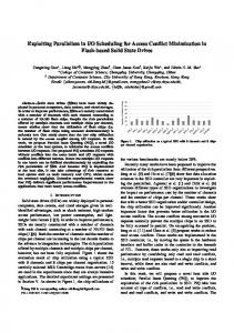
gram; thus we minimized the use of locking mechanisms. We saw the evaluation queue to be the main bottleneck of our implementation; we therefore chose to use a multiple-layered approach to simulate a single evaluation queue. Our approach is as follows.  Each processor uses a local evaluation queue. This queue is accessed locally and does not need to be locked. If the local queue has an element, it is evaluated rst. This queue is of xed length.  Each pair of two processors has a local/shared queue. If a processor's local queue is full, it places elements ready for evaluation on its local/shared queue. When a processor's local queue is empty, it rst searches its local/shared queue for the next element to be evaluated. This queue is shared and accessed via locking mechanisms.  If both a processor's local and local/shared queues are empty, then the local/shared queues of the remaining processors are searched in a round robin fashion. This scheme is illustrated in Figure 5. This approach led to promising results. The function p n T Ax X x x 1 + (1 + 2)bT x i f (x) = RT xi log 1 ? bT x ? p T log p 8b x 1 + (1 ? 2)bT x i=1 is the Helmholtz energy at the absolute temperature T of a mixed uid in a unit volume. Here R is the universal gas constant, and 0  x; b 2 Rn; A = AT 2 Rnn: This function and its gradient are used extensively in the simulation of oil reservoirs. Computing the gradient of the Helmholtz energy function with 300 independent variables, we were able to execute it over 11 times faster using 15 processors than using a single processor. We obtained similar results for up to 18 processors on the Sequent Symmetry. Figure 6 plots our results with respect to the theoretical linear speedup in the number of processors used.

4 Work in Progress

Our main concern at the moment is to develop a more ecient schedule for the parallel evaluation of the function and its derivatives using the reverse mode of automatic dierentiation. We are working on improving the eciency of parallel automatic dierentiation in several ways:  To increase the granularity of parallelism,  to decrease the synchronization overhead for locking queues and nodes in the computational graph, 5

Shared Queue

Shared Queue

PE

PE

PE

Local Queues

Shared Queue

PE

PE

Local Queues

....

PE

Local Queues

Run Time Ratio (Time Using 1 processor / Time Using N processors)

Figure 5: Simulating a Global Evaluation Queue

18 17 16 15 14 ADOL-C Implementation

13 12

Linear Speedup

11 10 9 8 7 6 5 4 3 2 1 0 0

1

2

3

4

5

6

7

8

9

10

11

12

13

14

15

16

Number of Processors Used

Figure 6: Parallel Test Results vs. Linear Speedup

6

17

18

 to decrease storage requirements.

formed in a subroutine is signi cantly higher than the number of input and output arguments. Secondly, we can use whatever method is best suited for evaluating G and its rst derivatives. If G can make use of user- or vendor-supplied optimized routines, or has been parallelized itself, we will exploit this eciency in a transparent fashion. The same applies to the computation of the derivatives. If we know a closed form for G0(x), or have an optimized, and perhaps parallelized code for computing G0(x), we can exploit it. This also would allow for selective tuning of performance-critical subroutines: We write by hand code for the computation of the derivatives of simple, but compute-intensive functions, and let ADOL-C take care of the rest. Lastly, we must nd a way to exploit user intuition about parallelism. Currently, if we are evaluating a parallel do loop, we cannot capture the user's intuition that all the dierent iterations of the loop body could be done at the same time (and as a consequence, the corresponding forward and reverse passes through the loop body). Obviously, user-supplied parallelism can usually be exploited very advantageously, and with little synchronization overhead, and in the long run, we have to be able to capitalize on that information. We are currently working on an improved and portable implementation of our graph evaluation scheme using the P4 communication library that has been developed by Lusk et al. at Argonne National Laboratory. In order to decrease graph storage and processing overhead, we are working on incorporating the hoisting chains of nodes, eliminating dead roots and assignments. As a next step, we will then incorporate hooks for user-supplied subroutines, with vector and matrix operations as the rst choice, and also work on ways to incorporate user-supplied parallelism.

The small granularity of parallelism is a consequence of the fact that our dierentiation arithmetic deals only with elementary operations at a scalar level. This approach has the advantage that the run-time system needed to support automatic dierentiation is easy to implement, since it only has to support relatively few and simple operations. If we want to maintain this view, we could increase processing granularity by identifying subgraphs of the computational graph that have comparatively few edges crossing the subgraph boundaries (that is, we can look for good edge separators). Subgraphs thus de ned will be assigned to one processor and will be completely evaluated on this processor. Finding good edge separators is a hard problem, however, and the sheer size of the computational graphs that we are dealing with is likely to make this approach rather expensive. An in our view more promising approach is to increase the granularity of the operations that are part of our dierentiation arithmetic. The Helmholtz energy function is a good example. The loops in the computation of g(x) = xT Ax will be completely unrolled, resulting in O(n2) vertices for an n  n matrix A. The gradient rg(x) = 2Ax will then be evaluated by traversing those vertices, applying dierentiation arithmetic on O(n2 ) scalars in succession. This is a rather complicated way of computing a matrix-vector product. Since derivative information for the basic vector-vector and matrix-vector operations is known, we are much better o to make these operations part of our dierentiation arithmetic. The advantages are two-fold: we increase computation granularity by going from n scalar nodes to a supernode containing n scalar operations, and we tremendously decrease the storage required for either the tape or the graph. Note that the hoisting operation introduced in the preceding section applies to \vector nodes" as well. Vector nodes are a special case of an operation where we may rely on a system other than ADOL-C to produce the required derivative information. Assume for example, that the user program repeatedly (` times, say), calls a subprogram computing a function G : Rn ! Rm . In the current implementation, the computational graph will contain ` traces through G, one for each of the separate invocations of G. On the other hand, if we were to regard G as part of our dierentiation arithmetic, we really need (x`1 ; : : :; x`n), and the function values G(x)jx=(x1 ;:::;x ) (the Jacobian G0(x)jx=(x1 ;:::;x ) may be recomputed during the reverse pass). If we have this information, we can complete our pass through the computational graph, and treat g as an atomic operation. This extension is attractive for several reasons. For one, storage for the trace of the computation is likely to be decreased considerably, since usually the number of operations per`

`

Acknowledgments

We thank Brad Karp, James Hu, Shawn Reese, and Jay Srinivasan for their dedicated collaboration in this project.

References

[1] W. Baur and V. Strassen. The complexity of partial derivatives. Theoretical Computer Science, 22:317{330, 1983. [2] Christian H. Bischof. A parallel QR factorization algorithm with controlled local pivoting. Technical Report ANL/MCS{P21{1088, Argonne National Laboratory, Mathematics and Computer Sciences Division, 1988. [3] Christian H. Bischof and Per Christian Hansen. Structure-preserving and rank-revealing QR factorizations. Technical Report MCS-P100-0989,

` n

` n

7

Argonne National Laboratory, Mathematics and Computer Sciences Division, September 1989.

[15] J. E. Horwedel, B. A. Worley, E. M. Oblow, and F. G. Pin. GRESS Version 0.0 Users Manual. Technical Report ORNL/TM 10835, Oak Ridge National Laboratory, Engineering Physics and Mathematics Division, 1988. [16] M. Iri and K. Kubota. Methods of fast automatic dierentiation and applications. Technical Report Research Memorandum 87-0, Department of Mathematical Engineering and Instrumentation Physics, Faculty of Engineering, University of Tokyo, 1987. [17] David Juedes and Andreas Griewank. Implementing automatic dierentiation eciently. Technical Report MCS{TM{140, Argonne National Laboratory, Mathematics and Computer Sciences Division, 1990. [18] S. Linnainmaa. Taylor expansion of the accumulated rounding error. BIT, 16:146{160, 1976. [19] J. J. More. On the performance of algorithms for large-scale bound constrained problems. In T. F. Coleman and Y. Li, editors, Large-Scale Numerical Optimization. SIAM, 1991. [20] I. M. Navon and U. Muller. FESW { a niteelement Fortran IV program for solving the shallow water equations. Advances in Engineering Software, 1:77{84, 1979. [21] Paul E. Plassmann. The Parallel Solution of Nonlinear Least-Squares Problems. PhD thesis, Dept. of Applied Mathematics, Cornell University, 1990. [22] Paul E. Plassmann. Sparse Jacobian estimation and factorization on a multiprocessor. In T. F. Coleman and Y. Li, editors, Large-Scale Optimization, pages 152{179, Philadelphia, 1990. SIAM. [23] Alex Pothen and Padma Raghavan. Distributed orthogonal factorization: Givens and Householder algorithms. Technical Report CS{87{24, The Pennsylvania State University, 1987. [24] B. Speelpenning. Compiling Fast Partial Derivatives of Functions Given by Algorithms. PhD thesis, Department of Computer Science, University of Illinois at Urbana-Champaign, 1980. [25] O. Talagrand and P. Courtier. Variational assimilation of meteorological observations with the adjoint vorticity equation. i: Theory. Q. J. R. Meteorological Society, 113:1311{1328, 1987. [26] P. Werbos. Applications of advances in nonlinear sensitivity analysis. In Systems Modeling and Optimization, pages 762{777, New York, 1982. Springer Verlag.

[4] Christian H. Bischof and Brad N. Karp. Increasing the granularity of parallelism and reducing contention in automatic dierentiation. Technical Report MCS{TM{142, Argonne National Laboratory, Mathematics and Computer Sciences Division, November 1990. [5] D. G. Cacuci. Sensitivity theory for nonlinear systems. i. nonlinear functional analysis approach. Journal of Mathematical Physics, 22(12):2794{ 2802, 1981. [6] D. G. Cacuci. Sensitivity theory for nonlinear systems. ii. extension to additional classes of responses. Journal of Mathematical Physics, 22(12):2803{2812, 1981. [7] T. F. Coleman and J. J. More. Estimation of sparse Jacobian matrices and graph coloring problems. SIAM Journal on Numerical Analysis, 20:187{209, 1983. [8] Thomas F. Coleman. Large Sparse Numerical Optimization, volume 165 of Lecture Notes in Computer Science. Springer Verlag, 1984. [9] George F. Corliss. Applications of dierentiation arithmetic. In Reliability in Computing, pages 127{148. Academic Press, 1988. [10] John Dennis and Robert Schnabel. Numerical Methods for Unconstrained Optimization and Nonlin