Jul 26, 2009 - sions while running the nation over a period of fifty years. In addition to ..... Average performance of the experimental group in trial 3 drops to a.
Paper presented at the 27th International Conference of the System Dynamics Society July 26-30, 2009
Exploratory strategies for simulation-based learning about national development
Birgit Kopainsky1, Stephen M. Alessi2, Matteo Pedercini3, Pål I. Davidsen1
1
2
System Dynamics Group, Department of Geography, University of Bergen, Postbox 7800, 5020 Bergen, Norway
College of Education, University of Iowa, 370 Lindquist Center, Iowa City, IA 52242, United States 3
Millennium Institute, 2200 Wilson Boulevard – Suite 650, Arlington, VA 22201, United States
Abstract This study investigated an instructional strategy to improve learning a complex model in a system dynamics based learning environment. The instructional strategy required subjects to explore key variables by manipulating dynamic graphs. Design of the strategy was posited upon principles of reducing cognitive load, facilitating mental models, enhancing transfer, and managing risk. Eight students who received the exploration strategy subsequently made better policy decisions than nine subjects who did not receive the strategy. Furthermore, the former subjects exhibited better understanding of the model and how to manage it than did the latter subjects, based upon their verbal descriptions.
1
Introduction
Dynamic systems are difficult to understand and manage successfully. This is not only observable in very complex dynamic systems. People also have difficulty making decisions in fairly simple dynamic systems (1992; Funke 1991; Jensen 2005; Moxnes 1998; 2004; Rouwette et al 2004; Sterman 1989a; Sterman 1989b). Improved understanding and decision making require further development of instructional strategies for presenting computer simulations and designing simulation based games (interactive learning environments). Such strategies are usually applied when designing the user interface of an interactive learning environment and include explanations of observed behavior, giving hints before user actions, and giving feedback following user actions (Alessi 2000a). Another approach to instructional support is guiding users through prior exploration of the system they will manage later on in the interactive learning environment. Sawicka & Kopainsky (2008) provide preliminary evidence that prior exploration improves performance in the decision making stage. The typical logic of a simulation based task is that users study textual instructions which describe the structure of the system they are supposed to manage. Users then progress to a decision making interface (interactive learning environment) where they must solve the task presented in the instructions. The prior exploration strategy is based on the hypothesis that the option to explore the behavior of a system (the behavior resulting from the structure described in the instructions) before actually making decisions improves understanding and performance. The current evidence for the effectiveness of prior exploration described in Sawicka & Kopainsky (2008) is limited to one specific task (reindeer management, a one stock model) and to a rather small subject pool. In this paper we test whether prior exploration improves performance and understanding in systems with more than one stock. Since 2006 we have been developing and refining an Interactive Learning Environment to teach long-term economic and social development in developing nations. BLEND (the Bergen Learning Environment for National Development), its underlying model, and our initial pilot tests are described in more detail in Alessi et al (2008), and Kopainsky et al (forthcoming). Summarizing it briefly, participants in BLEND play the roles of government ministers (education, health, agriculture, transportation, and the finance and prime ministers) who make and revise budget decisions concerning investment, taxes, and borrowing over a 35 year period. They see the effects of their budget decisions in different national outcomes including economic (e.g., income, national debt, government revenue), social (e.g., population, literacy, life expectancy), and environmental (e.g., water quality and forests). The six ministers work simultaneously and interact (via an instant messaging system) as they make their decisions. The goal of BLEND is for users to experience and understand that national development processes are characterized by non-linear relationships, delays, feedback loops, and multiple sources of causation requiring long-term policy design across government ministries. The intended users are high-level government workers from developing nations engaged in planning activities such as annual budgets, medium-term expenditure frameworks, poverty reduction strategies and national development plans. Our initial pilot testing of BLEND indicated participants need much more guidance to make decisions in such a complex environment. That and the goal of replicating and furthering the results of Sawicka & Kopainsky (2008) required a much simplified version of the ILE in which specific instructional strategies could be compared under more controlled conditions. A simplified version of BLEND with only five key stocks and which allowed participants to manage the nation individually (rather than in conjunction with five other ministers) was created, based on Pedercini (2009).
___________________________________________________________________________________________________________________________________________________________
1
In this study we investigate the effects of an exploratory instructional strategy on both learners’ performance and understanding. Performance refers to the success of learners’ problem solving within the Interactive Learning Environment (ILE). In this ILE it is represented by their decisions concerning key economic and social policies and their impact on national outcome variables: per-capita income, the government’s available budget for development, resources (as a fraction of the maximum possible), the debt over Gross National Product ratio, the national debt, and overall capital. Good performance is a function of increasing per-capita income, keeping the national debt low, increasing capital, and so on. Performance is a measure of initial learning during the simulation as represented by how well users of the ILE could make investment decisions while running the nation over a period of fifty years. In addition to and in contrast to performance, we also measured understanding. While performance was a measure of initial learning, understanding was a measure of transfer, because the tasks and questions that measured understanding were different than the activities (exploration and decision making) within the ILE. It is a measure of near transfer in contrast to far transfer (Laker 1990) because the concepts are the same and the context is very similar. In contrast, a measure of far transfer would have, for example, applied the principles learned in the ILE to a very different context, such as running a business instead of running a nation. Understanding was measured by asking the participants to explain verbally how decision variables (such as education investment) affect outcome variables (such as per-capita income), to draw graphs showing how national development will progress over time, and to draw causal loop diagrams representing the cause-and-effect relationships between variables in the national economy, including loops and delays. Because our participants had some (and varying) prior knowledge about economics and national development issues, they wrote verbal descriptions and drew causal loop diagrams both before and after using the ILE, as will be explained more in the experimental design section. We tested the effectiveness of the prior exploration strategy in a laboratory experiment where users had to manage a virtual developing nation over a time period of 50 years. Half of the users (the control group) studied textual instructions and then proceeded directly to the decision making phase. The other half (experimental group) studied textual instructions and then could explore the behavior of the system step by step before proceeding to the decision making phase. In this paper we report on the results and implications of a pilot test with 18 system dynamics master students (9 in each group) at the University of Bergen in Norway. The results of this pilot study will be used to further develop different versions of BLEND that are used for capacity building with the intended users. The next section summarizes the theoretical background of our approach. We then describe the simulation model and the laboratory experiment in which we tested the effectiveness of prior exploration. The results section presents the experiment’s outcomes for performance and understanding. Finally, we discuss the implications of our findings for ILE design, theory and future research.
2
Theory and relevant literature
Our design of the exploratory strategy was based on four theoretical pillars. Those pillars are intended to help overcome significant problems for those learning about national planning. We now summarize those problems and the underlying multi-theoretical approach we have adapted towards their solution. Put simply, our previous experiences with learners working in a complex interactive learning environment (ILE) suggest that their progress is hampered by four barriers:
___________________________________________________________________________________________________________________________________________________________
2
1.
Complex models underlying the ILE impose too much load on their cognition.
2.
Learners need to, but often cannot, form an adequate mental model to support decision making.
3.
Each step (or activity) in the ILE must be applied (i.e., must transfer) to subsequent performance steps, but that transfer often is unsuccessful.
4.
When faced with important decisions (even in a simulation) learners often demonstrate the anxiety typical of risk (or loss) avoidance.
These four barriers require corresponding solution approaches, and several are suggested by previous theories or principles in the literature concerning simulation and game design. They are: 1.
The ILE should increase complexity gradually and in accordance with the learners’ performance.
2.
The ILE should provide opportunities (or cognitive models) to help learners form adequate mental models.
3.
The ILE should provide activities that, primarily by virtue of the similarity principle, will foster transfer.
4.
The ILE should provide relatively risk-free activities that facilitate decision making without anxiety and the errors it can induce.
We now explain these four barriers and our projected solutions in a little more detail.
2.1
Problem 1 and solution approach 1
That learners in complex ILEs (or other simulations, games, or situations) have difficulty is well documented for many years (e.g., Dörner 1980; Sterman 1994). In more recent years, Cognitive Load Theory has provided a clear theoretical explanation for the phenomenon (Sweller 2005). Learner’s difficulty in complex environments is exacerbated when cognitive load is high and alleviated when designers are able to decrease cognitive load. Designers can do that, most easily, by decreasing extraneous cognitive load, such as that due to the complexity of a user interface, without sacrificing the interesting and important details of the content itself (Sweller et al 1998). But what can designers do when the content that must be learned is innately and unavoidably complex? Research and principles from simulation design and instructional design in general suggest that complex content be sequenced beginning with simpler or more general parts and dynamically increased in complexity (e.g., Alessi 2000b; Reigeluth 1999; Bruner 1960). This research study compared learners who are provided with a simplified “exploratory” activity before encountering a more complex decision making phase of a simulation with learners who proceeded straight to the more complex decision making task.
2.2
Problem 2 and solution approach 2
According to mental model theory, people learning about a phenomenon or situation will form a model in their mind of what is important and how things work (Seel et al 2000; Doyle & Ford 1998). Such models can take many forms. Driving around a new city one forms a static pictorial image of its layout, a mental map. Encountering verbal information such as a story, one fits components of the story into slots such as the villain or the hero, motives, causes and conse___________________________________________________________________________________________________________________________________________________________
3
quences. With dynamic phenomenon such as climate change or economic cycles we form mental simulations. The problem is that when a model is wrong, even in simple details, the results can be catastrophic. If your mental map of a city has north and south reversed, you’ll be lost. Even when not right or wrong, details of the learners’ model can have dramatic effects on performance. In a famous study of schema theory (assuming for a moment that mental models are types of schema), Pichert & Anderson (1977) demonstrated that when reading a description of a house, students remembered very different details depending on a single word in their directions -- whether they were told “imagine you are a homebuyer” versus “imagine you are a burglar”. If students in a simulation-based interactive learning environment have errors in their mental model of the underlying actual model, performance in the ILE will very likely be severely hampered. Thus, it is imperative that we help students develop reasonably accurate mental models of the ILEs actual underlying model. The previously mentioned exploratory activity was designed not only to provide a gradual increase in complexity, but to facilitate good (even if simplified) mental model formation.
2.3
Problem 3 and solution approach 3
People frequently acquire knowledge yet fail to transfer it to applicable situations. We commonly think of transfer of learning as referring only to the use of what we learn in some “real world” situation (Lobato 2006). But much more basically, transfer of learning is simply being able to apply whatever we have just learned at the present time for activity at some later time. That later time may be five minutes later. For example, if a student sets parameters in a system dynamics model and observes a particular outcome, using that just-acquired knowledge to do the next simulation run with sensible parameter choices (such as to test a new hypothesis) is an example of transfer, albeit very short term and near transfer. Learning something yet failing to transfer that knowledge is all too common, especially when the activity is complex and the student does not see the relevance of what was just learned to the next step. A key principle of near learning transfer is the similarity principle (Gagné 1954; Osgood 1949), which says that the more similar the stimuli and responses of two situations are, the more likely transfer of learning will occur. In contrast, far transfer, which has been likened to generalization in learning, is more dependent on variation in situations, stimuli and responses (Barnett & Ceci 2002). Because we are dealing much more with near transfer, the similarity principle suggests our solution approach to combat Problem 3. As designers, we must provide learning activities in an ILE that are clearly applicable (evidenced by their similarity) to the ultimate learning goals of the ILE. Thus, the variables that we encourage students to explore in the exploratory phase of our experiment are the same variables they will make decisions about in planning a national economy, their ultimate learning goal.
2.4
Problem 4 and solution approach 4
Risk taking is an individual difference with wide variations. Yet even though people vary greatly in their willingness to take risks, most people tend to decrease their risk taking when they perceive the stakes as being high (e.g., dangerous or potentially very expensive) and increase their risk taking when the stakes are low (nothing much will happen). Kermer et al (2006) suggests that people will avoid losses unless they perceive the amount of potential gain as much greater (perhaps twice as much) than the amount of potential loss. But a key word in the last sentence is perceive, because it is not actual danger or cost that drives people so much as what they believe the danger or cost may be. As an example, it is well known that people are more afraid of travel in airplanes than in cars, even though the chances of an accident are much greater ___________________________________________________________________________________________________________________________________________________________
4
in the car. Kermer et al (2006) also pointed out that people expect the emotional effect of losses will be much greater than they in fact turn out to be. In previous pilot tests of our ILE, we have observed that participants fear of making decisions which might bankrupt their nation make them extremely nervous and risk averse. They tend to make decisions they believe are conservative and safe (such as lowering taxes), even though such choices may in fact not be the wisest. Despite it just being a simulation or a game, learners perceive the ultimate outcomes (a successful nation versus a failed nation) as too important to take chances with. Just as Hamlet approached his problem (determining who killed his father) with “a play within the play”, our solution approach to Problem 4 is to provide a simulation within the simulation. Our experimental subjects’ exploratory phase allows them to just “play around with” some of the nation’s critical economic variables (such as the government’s health care expenditures and education expenditures) before they “actually run” the country as the Prime Minister. Of course, it is all make believe. Nevertheless, participants perceive the playing around simulation as safe compared to the subsequent running the country simulation, which they perceive as too important to fail.
2.5
Implications for method
In summary, based on these four problems and solution approaches, we designed a simulation exploratory phase to precede the simulation decision making phase. The exploratory phase had four critical design features. First, it started with reduced complexity so as to minimize initial cognitive load, gradually increasing complexity so as to avoid sudden cognitive overload. Second, it was designed to induce a good mental model of how key economic input variables (expenditures) affected economic and social outcome variables (income). Third, it was designed to foster good transfer of learning by maintaining as much similarity as possible between the situations and activities of the exploratory phase and the decision making phase. Fourth, the exploratory phase was designed to be perceived as more “safe” than the decision making phase, so as to encourage exploratory behavior, even potentially risky exploration, because it is necessary for participants to see what can bankrupt a nation in order to later avoid bankrupting their nation.
3
Simulation model
The simulation model used for the task is based on an extensive, model-based cross-country analysis that identified the role of a country’s resources for its long term economic development (Pedercini 2009). The model depicts the development of per capita income over time as a consequence of reinforcing processes between capital accumulation through private sector development (R1) and capital accumulation through human development (R2 and R3; Figure 1). All variables are calculated on a per capita basis (e.g. capital per capita, debt per capita, and government development budget per capita) so that demographic development does not have to be taken into account. Income per capita is equivalent to per capita production and production is driven by the available physical capital (machinery, equipment and buildings) and by total factor productivity. A country’s government cannot invest in physical capital directly. However, it can improve the general investment environment by investing in education, health and roads (education/health/roads expenditure). Investors in capital will invest the potentially available money (a share of per capita income) more when the labor force is more productive (i.e. more skilled and physically healthier) and roads provide access to input (from suppliers) and output markets for the goods produced.
___________________________________________________________________________________________________________________________________________________________
5
Per capita income feeds the government development budget through taxes. The government development budget is the budget that is available for investment in education, health and roads and thus closes a series of reinforcing feedback loops between per capita income and the three resources education, health and roads. The accumulation process of the education, health and roads resources establishes a number of balancing mechanisms that are not shown in Figure 1. The three resources cannot grow beyond their maximum value. The closer a resource gets to its maximum value the slower the stock grows. In the case of education, the maximum value is an adult literacy rate of 100%. For health it is 100% access to basic health care and for roads it is a roads density comparable to the kilometers of roads per person in the year 2000 in the United States. Figure 1: Reinforcing relationships between per capita income and the three production resources education, health, roads +
capital investment +
capital
+ R1 investment environment ++ +
+
+ per capita income
R2 +
education+
productivity +
R3
+ education expenditure
health
+
health expenditure
+
+ government development budget
+
+ roads
+
roads expenditure
Every five years, as part of a national development planning effort, the subjects decide on the expenditures for education, health and roads. They can do three things: 1.
Distribute more than the total available development expenditure. In this case they borrow money and create a deficit.
2.
Distribute less than the total available development expenditure. In this case they will have a surplus and be able to service debt or lend money.
3.
Distribute the total available development expenditure without creating either a deficit or surplus.
The option to borrow money creates an additional reinforcing feedback loop (Figure 2). Borrowing adds to the country’s debt and thus to interest payments on debt. Interest payments reduce the government development budget and, in the absence of other processes, create a need for borrowing even more money if expenditure levels are to be kept at high levels. The initial conditions are such that the country has no debt at all, that is, a balanced budget. The full stock and flow diagram as well as model equations are reproduced in Appendix 3.
___________________________________________________________________________________________________________________________________________________________
6
Figure 2: Reinforcing relationship between government development budget and debt
education + expenditure + health expenditure
roads expenditure
government development budget
-
+ + + +
interest payments on debt +
R -
debt +
borrowing
The simulation model was built using Vensim®. The user interface for the experiment was designed in VenappTM.
4
Experimental design
4.1
Task and decisions
Subjects play the role of the prime minister in Blendia, a virtual sub-Saharan African Nation which, at the outset, is one of the poorest nations in the world (per capita income of $300 per person per year). Their task is to achieve and maintain the highest possible per capita income in the course of 50 years. Long-term planning efforts in developing countries span a time period of about 15 years for the formulation of development strategies and about 40 years for the formulation of development visions. The time horizon of 50 years is also necessary because of the long time delays involved in the accumulation of human resources (it takes about two decades for investment decisions to cause considerable differences in the development pattern of the country). Behavior patterns such as worse-before-better or better-before-worse only become visible with such a long time horizon. The prime minister has far reaching financial responsibilities and the absolute power to make the following decisions:
•
Investment in education (explicit decision)
•
Investment in health (explicit decision)
•
Investment in roads (explicit decision)
•
Borrowing to finance such investments (implicit decision resulting from the three previous ones).
Investment and borrowing decisions are made every five years. The simulation starts in equilibrium and the prime minister stays in office throughout the 50 years no matter how poor his or her performance.
___________________________________________________________________________________________________________________________________________________________
7
4.2
Optimal solution
Optimal performance Optimal performance results from decisions that take the following issues into account and thus avoids undesirable impacts of well-intentioned investment policies: •
Balancing of the three production resources: Neither roads, health or education alone can stimulate per capita income very much. Total factor productivity and the investment environment grow fastest when the three production resources are balanced. Throughout the simulation horizon it is therefore important to monitor the development of the three production resources and develop them in a balanced way.
•
Delays of different durations: Investments in education take a long time to have visible effects on per capita income. Knowledge, skills, techniques and capabilities embodied in labor can be acquired through education and training but they require time to become effective. The same holds true for investments in health. The time necessary to achieve improvements in average life expectancy is, however, considerably shorter than the time required to increase the average adult literacy rate (a proxy for education). The results of investment in roads becomes visible fairly soon. In order to stimulate a balanced growth, the optimal strategy is to prioritize in the early years those interventions that have the longest implementation time.
•
Accumulations: At the outset, it is very effective to borrow money and use it to boost the development of the three production resources. However, borrowing adds to debt which is a stock. With increasing debt, interest payments increase and these payments are deducted from tax revenue every year. Too aggressive borrowing or borrowing over too long a time period can easily bankrupt the country and destroy any improvements in per capita income. With reasonable debt in the early years and adequate allocation to education, health and roads, the economy starts growing so well that debts can be paid back and spending can be increased even more in all three budget categories. This allows users to heavily increase per capita income without having the negative effects of debt and interest payments.
The optimal quantitative values for each budget category and decision period were calculated using Vensim®’s policy optimization algorithm
Optimal understanding Optimal understanding is characterized by the following elements: •
Subjects are able to identify all the relevant variables in the instructions.
•
They are able to identify the relationships between the variables.
•
They are able to assign polarities to the relationships.
•
They are able to infer the characteristics of successful investment strategies described in the optimal performance section (above).
___________________________________________________________________________________________________________________________________________________________
8
4.3
Treatments
This paper analyzes the effectiveness of an exploratory instructional strategy on both learners’ performance and understanding. Our control group studied written instructions about the task and then proceeded directly to the decision making phase. The experimental group has the option to explore the behavior of the system described in the instructions (exploration phase) before actually making decisions (decision making phase) (see Figure 3). Figure 3: Experimental and control group Decision making phase
Instructions
Exploration phase
Control group
Textual
Experimental group
Simulation based
Experimental group The instructions (Appendix 1) described the structure of the simulation model underlying the experiment and the decisions subjects could make. During the exploration phase subjects could first explore the effect of each explicit decision variable in isolation and then explore the combined effect of all three decisions together: •
Step 1: The subjects could move a slider for the desired education expenditure up or down and observe the effect of any change in education expenditure in Year 0 (and thus in surplus or deficit) on the behavior of a series of indicators over the entire 50 years time horizon (Figure 4). Technically, the model is run in Vensim®’s SyntheSim mode so that the slider can be varied freely and the effects are instantly visible. The other expenditure categories are held constant at their initial levels.
•
Step 2: The subjects could move a slider for the desired health expenditure up or down.
•
Step 3: The subject could move a slider for the desired roads expenditure up or down.
•
Step 4: The subjects could move all three sliders and thus vary the expenditures for education, health and roads at the same time.
After each step the subjects were asked to note their observations and to explain the resulting behavior (see section 4.5 for more details on the questionnaires accompanying the simulation based tasks). This stepwise procedure forced subjects to experience the different delays of the three production resources both in isolation and together, as well as the dynamics of debt accumulation. The procedure also increased the intrinsic difficulty of the task step by step. In the exploration phase, the simulation model experiences a single step change in the three decision variables at year zero and not with changes in the decision variables every five years, as is the case during the decision making phase. In this way we hoped to facilitate a risk free, rich exploration that helps form an accurate mental model of the underlying system. However, we wanted to avoid revealing the optimal strategy too explicitly. The optimal strategy must be deduced in ___________________________________________________________________________________________________________________________________________________________
9
the decision making phase where the decisions are similar albeit not identical to the one-time decisions in the exploration phase. After the exploration phase the experimental group proceeds to the decision making phase and experiences three trials for solving the task. All three trials are with the same simulator. It is important to emphasize that the interface shown in Figure 4 uses dynamic graphs. As users move the slider (in the case of Figure 4 the desired budget for education) the graphs at the bottom of the page (e.g. per capita income - interest payments) change in accordance with the slider movement. Figure 4: User interface of step 1 in the exploration phase
pc income – intererest payments
debt over GDP (years)
government development budget
resources relative to maximum
deficit (-) or surplus (+)
capital
Control group The control group proceeded directly to the decision making phase after studying the instructions. Like the experimental group, the control group had three trials to solve the task. All three trials are with the same simulator. The interface for the decision making phase is shown in Figure 5. The situation shown in the figure is the initial situation with initial budget values but without any decisions made yet. Consequently, the graphs at the bottom of the figure are empty.
___________________________________________________________________________________________________________________________________________________________
10
Figure 5: Interface for the decision making phase
pc income – intererest payments
debt over GDP (years)
4.4
government development budget
resources relative to maximum
deficit (-) or surplus (+)
capital
Hypotheses
Based on our theoretical framework and previous studies using prior exploration we expect subjects in the experimental group to perform better and to have better understanding of the system. Concerning performance, our null and alternative hypotheses are: HP_0: There is no difference between performance in the experimental group and the control group HP_1: Performance in the experimental group is better than in the control group Concerning understanding, our null and alternative hypotheses are: HU_0: There is no difference between understanding in the experimental group and the control group HU_1: Understanding in the experimental group is better than in the control group
4.5
Procedure
Subjects were assigned randomly to the experimental or control group. Before starting the task, all subjects received the same pre-briefing. Pre-briefing emphasized that the subjects were about to manage a virtual nation over a rather unrealistic (that is, very long) time horizon. They were then given the general schedule of the experiment. Subjects were also told that they could make decisions and observe the impact of their decisions in the time graphs. The general logic of the budgeting process was also briefly discussed during the pre-briefing session. The subjects proceeded at their own self-paced speed and required between 60 and 90 minutes to complete the experiment. Each subject had three trials during the decision making phase. The experimental session ended with a plenary debriefing session which included an exchange of experiences during the experiment, collaborative development of the underlying model structure and a discussion of the short and long term effectiveness of different investment strategies. ___________________________________________________________________________________________________________________________________________________________
11
In addition to the simulation based activities, subjects completed several questionnaires designed to explain their performance and assess their understanding of the system (the questionnaires are reproduced in Appendix 2). After subjects were introduced to the nation of Blendia (the instructions) but before engaging in any simulation activities (either exploration for the experimental group, or decision making trials for both groups), all subjects were asked several questions on a questionnaire. They were asked: 1.
How well they understood the task (subjective understanding of the task, multiple choice). Answers to this question will be used to control for prior knowledge that might affect subject performance or understanding.
2.
To draw a causal loop diagram depicting the economy of Blendia (pre-simulation system description). In subsequent versions of this paper metrics for understanding will be developed to evaluate answers to this question.
3.
To describe the strategy they planned to pursue regarding government policy decisions and draw graphs of how they believed those policies would affect key variables over time (presimulation strategy description). In order to evaluate answers to this question metrics for understanding are developed in section 5.2.
After engaging in all simulation activities (both exploration and decision making trials) all subjects were again given a questionnaire. They were asked: 1.
To describe any unexpected behavior in the simulation and how it could be explained,
2.
To once again draw a causal loop diagram depicting the economy of Blendia (postsimulation system description). In subsequent versions of this paper metrics for understanding will be developed to evaluate answers to this question.
3.
To again describe the strategy they would pursue regarding policy decisions and how they would affect key outcomes for Blendia if they were given an additional trial (post-simulation strategy description). In order to evaluate answers to this question metrics for understanding are developed in section 5.2.
4.
They were also asked five questions regarding their interest in, prior knowledge of, and experience with national development issues and the use of simulations for national planning (demographic data). Answers to these questions will be used to control for demographic effects on subject performance and understanding.
Subjects in the experimental group also answered one question after each exploration step. After observing the reaction of key indicators to changes in expenditures, subjects were asked to write down their observations of what had happened to per capita income and other indicators when they had changed the expenditures and why they thought this had happened. According to Dörner (1996) opportunities for reflection contribute to improving understanding. This pause after each exploration stage provided the learners with an opportunity to reflect and avoids the impression that they are just manipulating parameters. The expectation is that learners eventually gain an appreciation for the complexities of the system (Spector et al 2001). These questions, and the reflection they induced, were intended as part of the instructional strategy, and not a measurement of outcomes.
___________________________________________________________________________________________________________________________________________________________
12
4.6
Subjects
Subjects were recruited from students with varied backgrounds who took a class in interactive learning environments as part of the international Masters degree program in System Dynamics at the University of Bergen in Norway. We ran the pilot experiment in January 2009 with nine subjects per group (n=9 for experimental group and n=9 for control group). The person in each group getting closest to the optimal solution in the shortest time (over trials) was promised and received a price. Each subject worked at a separate computer with no communication allowed with other subjects.
5
Performance and understanding assessment
5.1
Metrics of performance
Subjects were told to try to achieve and maintain the highest possible per capita income over the 50 years time horizon. We therefore evaluate performance by subtracting interest payments on debt from per capita income and comparing this value to the benchmark value. Performance can be evaluated based on two criteria: •
Shape of the curve relative to shape of the optimal curve. Effective long term strategies result in moderate per capita income growth in the short term because education resources need to be built first. The shape of the curve therefore gives insight into the time horizon over which a subject formulates their strategy.
•
Distance to optimal value (optimal values over time, respectively). The distance to the optimal value, either for the last year or for the entire simulation horizon allows for statistical analysis of experimental and control group’s performance and the difference between the two.
5.2
Scoring protocol for understanding
Subjects’ understanding after using the simulations was initially assessed using the questions about their policy strategies, which had been asked both before and after using the simulation (the pre- and post-simulation strategy description). Although those questions included drawing pictures, we have analyzed only the textual descriptions by the subjects, which were much more complete and clear. These textual descriptions were compared for the experimental subjects (those who engaged in the exploratory activity before the decision making trials) and the control subjects (those who did not have the exploratory activities). The responses of the experimental and control subjects were printed on one side of an index card and their subject number (including condition) was on the reverse side to enable blind scoring. A scoring protocol was devised and is as follows. Subjects received one point if their description included the concept of balancing the key expenditures (education, roads, and health). They received one point as well if their description included the concept of long delays between investments and desired outcomes. They received one point as well if their description included education and roads requiring early investment. Finally, they received one more point if they included the notion that at a later time, debt should begin to be paid off. This scoring was fairly liberal, that is, any phrase suggesting they understood these key concepts was awarded a point, for either condition, such as if they said, “the country will be paying off debts accumulated over the first six years.”
___________________________________________________________________________________________________________________________________________________________
13
In addition to the points for correct concepts in their description, we separately kept track of explicitly incorrect concepts in their descriptions. The only two explicit errors we found for any subjects were (1) suggesting that debt be paid off at the beginning and (2) saying that education and roads be invested in at the end. Again, this scoring was fairly liberal. An error was counted if the subject said anything suggesting they had a misconception, such as, “I would invest more in the end.”
6
Results
6.1
Performance
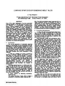
Figure 6 presents the results of the experimental design with the experimental and control group. The grey line represents the optimal solution while average performance in the three trials is shown by the three black lines.1 In trial 1 and 2 the experimental and the control group show considerable differences. Average performance of the experimental group in trial 3 drops to a negative value. This is caused by two subjects who in the previous two trials performed well and apparently tried out a completely new strategy in trial 3. Without these two subjects the average performance in trial 3 is marginally higher than in trial 1. Average performance in the experimental group throughout the trials (with the two subjects omitted from trial 3) shows continuous improvements in per capita income minus interest payments. The average behavior pattern for the control group, on the other hand, is an initial slight growth followed by a decline that is caused by high interest payments. Performance over trials improves slightly but the shape of the curve remains the same. Figure 6: Optimal and average performance of the experimental and control groups control group
1500
1500
1250
1250 pc income - interest payments
pc income - interest payments
exploration group
1000 750 500 250 0 0
5
10
15
20
25
30
35
40
45
50
1000 750 500 250 0 -250
-250 -500 0
-500 T1
T2
T3
optimum
5
10
15
20 T1
25 T2
30 T3
35
40
45
50
optimum
Figure 7 shows individual subject results for trial 1 both for the experimental and the control group. The figure shows that the subjects in the experimental group all manage to steadily increase per capita income (corrected for interest payments on debt). The performance of the subjects in the control group, on the other hand, is more varied and reaches from fairly successful subjects to unsuccessful performers who buy high values of per capita income with high debt so that the per capita income corrected for interest payments becomes negative towards the end. It seems that the major impact of the prior exploration strategy is that the vicious cycle of the reinforcing debt loop can be avoided. 1
One subject in the experimental group had to be eliminated from the analysis for not following the instructions. An outlier is defined as a subject who clearly misunderstood the task. Answers in the questionnaires made it very clear that this particular subject had not understood what they were supposed to do. Subjects who bankrupted their country towards the end of the simulation were not eliminated. Instead, they are unsuccessful performers because they buy high values of per capita income with high debt.
___________________________________________________________________________________________________________________________________________________________
14
Figure 7: Overview of individual subjects’ results in trials 1 for the experimental and the control group control group
1500
1500
1000
1000 pc income - interest payments
pc income - interest payments
experimental group
500
0 0
5
10
15
20
25
30
35
40
45
50
-500
500
0 0
5
10
15
20
25
30
35
40
45
50
-500
-1000
-1000
-1500
-1500
To see if the differences are statistically significant we compared per capita income – interest payments for the two groups using a two-tailed unpaired t-test (Figure 8). The difference between the experimental and the control group was statistically significant on a 10% level (p=0.1) for the second half of the simulation period. At the outset, the two groups are fairly similar. Due to the long time delays involved in the accumulation of the human resources subjects’ decisions only have an observable effect on per capita income and per capita interest payments after about two decades. At this point in time the difference between the two groups becomes statistically significant. Hypothesis HP_0 (There is no difference between performance in the experimental group and in the control group) therefore must be rejected. Figure 8: p values for difference in performance in trial 1 1.00 0.90 0.80 0.70
p values
0.60 0.50 0.40 0.30 0.20 0.10 0.00 1
6
11
16
21
26
31
36
41
46
year
6.2
Understanding
After blind scoring we had two scores for each subject. The first was the number of correct concepts in their descriptions. Subjects ranged from 0 to 3 correct concepts. Nobody had all four correct concepts in their responses. The second score was the number of correct concepts minus the number of incorrect concepts. Those scores ranged from -1 to 3. None of the subjects gave both of the incorrect concepts, but half of the subjects (in each treatment) gave one or the other. The one subject who was not included in the analysis of performance data was also eliminated from the analysis of understanding. Means and two-tailed unpaired t-tests were calculated for both scores (Table 1).
___________________________________________________________________________________________________________________________________________________________
15
Table 1: Means and two-tailed unpaired t-tests for differences in understanding Score Number of correct concepts Number of correct concepts – number of incorrect concepts
Mean experimental group 1.75 1.25
Mean control group 0.75 0.25
Two-tailed unpaired t-test p=0.04 p=0.14
Significance (10% level) Significant Not significant
With the disclaimer that our scoring protocol was fairly liberal and the number of subjects was rather small, the results in Table 1 suggest that for correct statements of understanding, the subjects who engaged in exploration demonstrated better understanding than those who did not engage in exploration. Hypothesis HU_0 (There is no difference between understanding in the experimental group and in the control group) is therefore tentatively rejected.
7
Discussion and conclusions
Despite the small number of subjects, we found evidence that engaging subjects in exploration of important variables using dynamic graphs is an instructional strategy that improves their learning from a system dynamics-based interactive learning environment. This is true not only for initial learning (performance during the ILE), but also for transfer (evidenced by their understanding of the underlying model and how to manage it). Both performance and understanding were significantly better for the experimental group (those subjects who engaged in the exploratory activity before decision making trials) than for the control group (those subjects who did not have the exploratory activities). The significant difference in performance agrees with previous results (Langley & Morecroft 2004; Sawicka & Kopainsky 2008; Skraba et al 2007). More importantly, the experimental subjects’ improved performance appears to be for the right reasons, given that they exhibited better understanding. The experimental subjects’ improved understanding can also be interpreted as greater near transfer of learning than the control subjects. That transfer was from the activities of the simulation (both exploration and decision making trials) to a different (though similar) use of the knowledge, being able to verbally explain the model and how to manage it. Better understanding in the experimental group is important because the instructional strategy (providing guided prior exploration) must improve the rules governing decision making in order to be considered an effective instructional strategy. Improved performance should not be a consequence of trial and error until a satisfactory constellation of decision variables is found, and without a fundamental appreciation for why these decisions should be implemented. The design of the prior exploration strategy was based on the hypothesis that the opportunity to explore a system’s behavior (that which results from the structure described in the instructions), and doing so before implementing policy decisions, improves understanding and performance. The literature provides ample evidence that people have great difficulties inferring behavior even from the simplest structures (e.g., Booth Sweeney & Sterman 2000; Moxnes & Saysel 2009; Sterman & Booth Sweeny 2007). The exploratory activities provided in this ILE did appear to help subjects learn the connection between the structure and behavior of this particular system. It should be pointed out that although some significant results were found, the evidence could have been stronger. Concerning our understanding data, it would have been nice for experimental subjects to not only identify more correct concepts (which they did) but also make fewer errors. Experimental and control subjects made equal numbers of errors.
___________________________________________________________________________________________________________________________________________________________
16
7.1
Implications of our study for ILE design
The purpose of this study was not only to replicate and extend the results of Sawicka & Kopainsky (2008), but to develop improved instructional strategies for the interactive learning environment we have been working on since 2006. As others have pointed out (de Jong & van Joolingen 1998) and as we have observed in our ILE pilot testing (Alessi et al 2008), students in simulation-based learning environments need instructional support. Without it, most students engage in unproductive trial and error learning. Furthermore, there is evidence that simply providing opportunities for exploration or other learning strategies tends to be ineffective because students fail to take full advantage of them (Größler et al 2000). We therefore implemented an instructional strategy in which students were explicitly presented with an exploratory learning tool, though the time and effort they expended with the tool was up to them. The exploratory learning tool was designed to make the relationships between important variables visually clear through dynamic graphs, and to do so in a way that was risk free for the students. Students in simulation-games often put a priority on winning (or doing well in the eyes of other people) rather than on learning as much as they can, and our exploratory learning tool allowed them to explore structure-behavior relationships before the game started and performance became more important. Our results do not allow us to separate the contribution of these various factors. But it does appear that this particular technique of requiring use of a risk-free visual exploratory tool is effective.
7.2
Implications for theory
Our study and the experimental instructional strategy (exploring important variables with dynamic graphs) were based on four theory-based principles. First, cognitive load theory and the often identified difficulty students have with complex activities or learning environments suggests gradually increasing complexity. Not only was the exploratory activity of less complexity than the policy decision making part of the simulation, but the exploratory activity was itself sequenced from easier to more difficult information. Second, mental model theory suggests providing cognitive models (e.g., computer animations) to help students form accurate and useful mental models. The dynamic graphs are such a cognitive model. This cognitive model visually and persuasively demonstrates key relationships in the underlying simulation model. Third, transfer of learning theory suggests using the similarity principle to foster near transfer from one concept or activity to very similar new concepts or activities. Although the exploratory activity was simpler than the policy decision making activity, it involved the same variables within the same context (the dynamics of a national economy). Fourth, risk and loss avoidance theory suggests that people overestimate the emotional impact of loss and so overreact in the desire to avoid losses in risky situations. The exploratory activity was designed as a risk-free activity and should thus induce more worry-free exploratory behavior on the part of learners. Our simple experimental design and small number of subjects could not provide data to separate the contribution of these four theoretical positions. But it would appear some combination of them does serve to improve students’ performance and understanding of complex relationships in a system dynamics-based learning environment.
___________________________________________________________________________________________________________________________________________________________
17
7.3 Limitations of the current study and implications for future research Experimentally, the greatest limitation of the current study is that control students can be viewed as receiving less instruction than the experimental students. An alternative task for the control students would eliminate the possible explanation that experimental students had more instruction or simply more time on task. A possible alternative task is to have the control students read a text about the relationships between key variables. Future research will include that or some other intervening task (between the instructions and the policy decision making trials). More subjects would not only permit greater statistical power for the analyses we did perform, but would allow other interesting analyses such as the correlation between performance and understanding, and perhaps between the degree of exploration (since students could manipulate the sliders and observe the dynamic graphs as much or as little as they wanted) and the outcome variables (performance and understanding). As guided exploration seems to be effective in terms of understanding and performance it would be useful to analyze in more depth what kind of exploration is most effective. After a research study one always realizes additional things one could have done. In our case, we realized it would have been nice to assess understanding immediately after exploration (for students in the experimental condition) and perhaps after each of the performance trials.
8
References
Alessi SM. 2000a. Designing educational support in system-dynamics-based interactive learning environments. Simulation & Gaming 31:178-96 Alessi SM. 2000b. Simulation design for training and assessment. In Aircrew training and assessment, ed. HF O'Neil Jr., DH Andrews, pp. 497-509. Mahwah, NJ: Lawrence Erlbaum Associates Alessi SM, Kopainsky B, Davidsen PI, Pedercini M. 2008. A system dynamics-based multi-user domain for improving national development planning. In Annual Meeting of the American Educational Research Association. New York City, NY Barnett SM, Ceci SJ. 2002. When and where do we apply what we learn? A taxonomy for far transfer. Psychological Bulletin 128:612-37 Booth Sweeney L, Sterman JD. 2000. Bathtub dynamics: initial results of a systems thinking inventory. System Dynamics Review 16:249-86 Brehmer B. 1992. Dynamic decision making: Human control of complex systems. Acta Psychologica 81:211-41 Bruner JS. 1960. Process of education. New York: Vintage Books de Jong T, van Joolingen WR. 1998. Scientific discovery learning with computer simulations of conceptual domains. Review of Educational Research 68:179-201 Dörner D. 1980. On the difficulties people have in dealing with complexity. Simulation & Games 11:87-106 Dörner D. 1996. The logic of failure. New York: Metropolitan Books/Henry Holt Doyle J, Ford D. 1998. Mental models concepts for system dynamics research. System Dynamics Review 13:253-65
___________________________________________________________________________________________________________________________________________________________
18
Funke J. 1991. Solving complex problems: Exploration and control of complex systems. In Complex problem solving: principles and mechanisms, ed. R Sternberg, P Frensch, pp. 185-222. Hillsdale, NJ: Lawrence Erlbaum Gagné RM. 1954. Training devices and simulators: Some research issues. The American Psychologist 9:95-107 Größler A, Maier FH, Milling PM. 2000. Enhancing learning capabilities by providing transparency in business simulators. Simulation & Gaming 31:257-78 Jensen E. 2005. Learning and transfer from a simple dynamic system. Scandinavian Journal of Psychology 46:119-31 Kermer DA, Driver-Linn E, Wilson TD, Gilbert DT. 2006. Loss aversion is an affective forecasting error. Psychological Science 17:649-53 Kopainsky B, Pedercini M, Alessi SM, Davidsen PI. forthcoming. A blend of planning and learning: Simplifying a simulation model of national development. Simulation & Gaming Laker DR. 1990. Dual dimensionality of training transfer. Human Resource Development Quarterly 1:209-23 Langley PA, Morecroft JDW. 2004. Performance and learning in a simulation of oil industry dynamics. European Journal of Operational Research 155:715-32 Lobato J. 2006. Alternative perspectives on the transfer of learning: History, issues, and challanges for the future. The Journal of the Learning Sciences 15:431-49 Moxnes E. 1998. Not only the tragedy of the commons: Misperceptions of bioeconomics. Management Science 44:1234-48 Moxnes E. 2004. Misperceptions of basic dynamics: the case of renewable resource management. System Dynamics Review 20:139-62 Moxnes E, Saysel AK. 2009. Misperceptions of global climate change: information policies. Climatic Change 93:15-37 Osgood CE. 1949. The similarity paradox in human learning: A resolution. Psychological Review 56:132-43 Pedercini M. 2009. Modeling resource-based growth for development policy analysis. Doctoral thesis. University of Bergen, Norway, Bergen Pichert JW, Anderson RJ. 1977. Taking different perspectives on a story. Journal of Educational Psychology 69:309-15 Reigeluth CM. 1999. The elaboration theory: Guidance for scope and sequence decisions. In Instructional Design Theories and Models: A New Paradigm of Instructional Design, ed. CM Reigeluth, pp. 425-53. Mahwah, NJ: Lawrence Erlbaum Associates Rouwette EAJA, Größler A, Vennix JAM. 2004. Exploring influencing factors on rationality: a literature review of dynamic decision-making studies in system dynamics. Systems Research and Behavioral Science 21:351-70 Sawicka A, Kopainsky B. 2008. Simulation-enhanced descriptions of dynamic problems: Initial experimental results. In 26th International Conference of the System Dynamics Society. Athens, Greece Seel NM, Al-Diban S, Blumschein P. 2000. Mental models and instructional planning. In Integrated and holistic perspectives on learning, instruction and technology: Understanding complexity, ed. JM Spector, TM Anderson. Dordrecht, The Netherlands: Kluwer Skraba A, Kljajic M, Borstnar M. 2007. The role of information feedback in the management group decision-making process applying system dynamics models. Group Decision and Negotiation 16:77-95 Spector JM, Christensen DL, Sioutine AV, McCormack D. 2001. Models and simulations for learning in complex domains: using causal loop diagrams for assessment and evaluation. Computers in Human Behavior 17:517-45
___________________________________________________________________________________________________________________________________________________________
19
Sterman JD. 1989a. Misperceptions of feedback in dynamic decision making. Organizational Behavior and Human Decision Processes 43:301-35 Sterman JD. 1989b. Modeling managerial behavior: Misperceptions of feedback in a dynamic decision making experiment. Management Science 35:321-39 Sterman JD. 1994. Learning in and about complex systems. System Dynamics Review 10:291330 Sterman JD, Booth Sweeny L. 2007. Understanding public complacency about climate change: adults' mental models of climate change violate conservation of matter. Climatic Change:213-38 Sweller J. 2005. Implications of cognitive load theory for multimedia learning. In The Cambridge handbook of multimedia learning, ed. RE Mayer, pp. 19-31. Cambridge, UK: Cambridge University Press Sweller J, van Merrienboer JJG, Paas FGWC. 1998. Cognitive Architecture and Instructional Design. In Educational Psychology Review, pp. 251-96: Kluwer Academic Publishing
___________________________________________________________________________________________________________________________________________________________
20
Appendix Appendix 1: Instructions You have just been elected the Prime Minister of Blendia. You will stay in office as prime minister for a period of 50 years. You are thus in charge of the long term development of Blendia. Blendia is an island located off the western cost of Africa. It is currently one of the poorest countries in the world with an income per capita of 300 $ per year. Your task is to bring your country onto a sustainable economic growth path and achieve and maintain the highest possible income per capita. Income per capita results directly from production and production is driven by the available capital (machinery and its technology level) as well as by total factor productivity. As a government you cannot invest in capital directly. However, you can improve the general investment environment. Investors in capital will invest the potentially available money (a share of per capita income) more when the labor force is more productive and roads provide access to input and output markets for the goods produced. You can specifically invest in the following three resources: •
Education Investments in education are used for building and maintaining schooling capacity, i.e. for building and maintaining schools, for training and paying teachers, as well as for paying books. Education is the stock of knowledge, skills, techniques, and capabilities embodied in labor acquired through education and training. These qualities are important for the labor force to understand and perform tasks, to properly use the available physical capital, and to efficiently organize the production process. Maximum or optimal education would mean an average adult literacy rate of 100% (maximum or optimal value for Human Development Index calculations).
•
Health Investments in health are used for building and maintaining basic health care services, i.e. for building and maintaining health care centers, for training and paying doctors and nurses, as well as for paying drugs. Health defines the strengths of the labor force and thus its capability to properly use the available physical capital and to efficiently organize the production process. Maximum or optimal health would mean an average life expectancy of 85 years (maximum or optimal value for Human Development Index calculations).
•
Roads Investments in roads are used for building and maintaining roads. Efficient and extended infrastructure allows faster and cheaper access to the market, broader access to information, and reliable access to the inputs required for production. Maximum or optimal roads would mean a value of kilometers of roads per person as in the year 2005 in the United States.
___________________________________________________________________________________________________________________________________________________________
21
Budget issues For making your investment decisions you will have to take a number of budget mechanisms into account. Your expenditures for education, health and roads are fed by two sources:
•
Revenue: Through taxation the government generates revenue from per capita income.
•
Borrowing: You can borrow money from foreign resources. If you borrow money you start accumulating debt. Each year you will have to pay interest on your debt.
Government development expenditure •
In Blendia, government development expenditure is the total revenue minus interest payments on debt.
Decisions Every five years, as part of a national development planning effort, you decide on the expenditures for education, health and roads. You can do three things and as the prime minister you have the absolute power to decide (see also Figure 1):
1.
Distribute more than the total available development expenditure. In this case you borrow money and create a deficit.
2.
Distribute less than the total available development expenditure. In this case you will have a surplus and be able to service debt or lend money.
3.
Distribute the total available development expenditure without creating neither deficit nor surplus.
Figure 1: Budget decisions mechanism with initial values Government development expenditure – Education expenditure – Health expenditure – Transportation expenditure Surplus (+)/deficit (-)
90 $ per person – 30 $ per person – 30 $ per person – 30 $ per person 0
Evaluation Your performance will be evaluated on the following basis: •
Income per capita: You should try to achieve and maintain the highest possible income per capita. The country’s official goal is a value of 600 $ per capita in 50 years from today.
•
Interest payments on debt: Per capita income can only be maintained if you have not accumulated excessive debt. At the end of the 50 years period the interest payments on debt in year 50 will be deducted from your income per capita in year 50.
___________________________________________________________________________________________________________________________________________________________
22
Appendix 2: Questionnaires The questionnaires listed below contain all the questions for the exploration treatment. For space reasons the blank spaces for writing answers were deleted from the original document and question P3 only contains a reduced number of time-indicator axes on which projections had to be drawn. The control group answered the same questions without the exploration workbook (questions E.1 to E.4).
Post instructions questionnaire Question P1: How well do you feel you have understood the task? I understood the task: � Fully
� Well
� Reasonably well
� Not very well
� Not at all
Question P2: Please shortly describe the situation presented in the instructions. Try to identify how your policy decisions affect per capita income, government development expenditure and other important issues described in the instructions. Diagram showing the main variables and linkages: Question P3: Outline shortly your strategy for increasing per capita income in Blendia without reducing government development expenditure. Which policy decisions are you going to implement? How do you think they will affect the development of Blendia over time?
time
time
___________________________________________________________________________________________________________________________________________________________
23
Exploration workbook Question E.1: What happened to per capita income and the other indicators when you changed the budget for education? Why do you think this happened? Please note your key observations Question E.2: What happened to per capita income and the other indicators when you changed the budget for health? Why do you think this happened? Please note your key observations Question E.3: What happened to per capita income and the other indicators when you changed the budget for roads? Why do you think this happened? Please note your key observations Question E.4: What happened to per capita income and the other indicators when you changed the budget for all three policy sectors? Why do you think this happened? Please note your key observations
Final questionnaire Question F1: Did any unexpected behavior occur when you were playing the game? How do you think can this unexpected behavior be explained? Question F2: After having played the game, how would you now describe the situation presented in the instructions? What are the linkages between your policy options and performance indicators such as per capita income and government development expenditure? You can either draw a new diagram or adapt the original description in question P2 using a RED pen Question F3: If you were to play the game again, would you choose a new strategy for increasing per capita income without reducing government development expenditure? Which policy decisions would you implement? How do you think they would affect the development of Blendia over time? Question F4: How interested are you in development issues? � Extremely
� Quite
� Some
� Not particularly
� Not at all
___________________________________________________________________________________________________________________________________________________________
24
Question F5: How would you rate your knowledge of development issues? � Very good
� Good
� Average
� Poor
� Very poor
Question F6: Do you have any practical experience in development work? � Yes
� No
Question F7: Have you ever used simulation and modeling to study or manage development issues? � Yes
� No
Question F8: Have you ever taken classes in development studies/development economics? � Yes
� No
Thank you very much for participating!!!
___________________________________________________________________________________________________________________________________________________________
25
Appendix 3: Stock and flow diagram and equations COST EFFECTIVENESS INITIAL CAPITAL OF CAPITAL PER CAPITA INVESTMENT ELASTICITY OF INVESTMENT TO Capital Per ENVIRONMENT Capita capital investment
INITIAL INVESTMENT ENVIRONMENT investment environment
change in education
target education
DESIRED BUDGET FOR EDUCATION
change in health
HEALTH INVESTMENT DELAY
Health Relative To Optimum
RESOURCES EFFECT TABLE
Roads Relative To Optimum
ELASTICITY OF PRODUCTIVITY TO ELASTICITY OF HEALTH INCOME TO total factor CAPITAL productivity per capita income
total desired budget per capita
change in roads
COST EFFECTIVENESS OF RESOURCE INVESTMENTS
PRODUCTIVITY TO ROADS
DESIRED BUDGET FOR HEALTH
target health
effect of roads on investment environment
ELASTICITY OF PRODUCTIVITY TO EDUCATION ELASTICITY OF
EDUCATION INVESTMENT DELAY
Education Relative To Optimum
effect of education on investment environment
effect of health on investment environment
PROPENSITY TO SAVE
capital depreciation
per capita savings
effect of investment environment on capital investment
relative investment environment
CAPITAL DEPRECIATION TIME
government development budget per capita
ROADS INVESTMENT DELAY DESIRED BUDGET FOR ROADS
target roads
TAX RATE surplus or deficit
borrowing
INITIAL PC INCOME
Debt Per Capita
pc income corrected for interest payments
paying back debt over gdp ratio interest rate
interest payment on debt
INTEREST RATE TABLE
(01)
FINAL TIME = 50 Units: Year The final time for the simulation.
(02)
INITIAL TIME = 0 Units: Year The initial time for the simulation.
(03)
SAVEPER = 1 Units: Year [0,?] The frequency with which output is stored.
(04)
TIME STEP = 0.0625 Units: Year [0,?] The time step for the simulation.
(05)
borrowing= IF THEN ELSE(surplus or deficit0 :AND: Debt Per Capita>0, surplus or deficit,0) Units: $/Year
(42)
pc income corrected for interest payments= per capita income-interest payment on debt Units: $/Year
(43)
per capita income= INITIAL PC INCOME*Capital Per Capita^ELASTICITY OF INCOME TO CAPITAL*total factor productivity Units: $/Year (44)
per capita savings= per capita income*PROPENSITY TO SAVE Units: $/Year
(45)
PROPENSITY TO SAVE= 0.04 Units: Dmnl
(46)
relative investment environment= investment environment/INITIAL INVESTMENT ENVIRONMENT Units: Dmnl
(47)
RESOURCES EFFECT TABLE( [(0,0)-(1,1)],(0.15,0),(0.3,0.6),(0.33,0.7),(0.36,0.75),(0.4,0.8),(0.449541 ,0.842105),(0.501529,0.885965),(0.565749,0.921053),(0.629969,0.947368),(0.685015 ,0.964912),(0.749235,0.97807),(1,1)) Units: Dmnl
(48)
ROADS INVESTMENT DELAY= 3 Units: Year
(49)
Roads Relative To Optimum= INTEG (change in roads, 0.3) Units: Dmnl
(50)
surplus or deficit= government development budget per capita-total desired budget per capita Units: $/Year
(51)
target education= MIN(DESIRED BUDGET FOR EDUCATION*COST EFFECTIVENESS OF RESOURCE INVESTMENTS, 1) Units: Dmnl ___________________________________________________________________________________________________________________________________________________________
29
(52)
target health= MIN(DESIRED BUDGET FOR HEALTH*COST EFFECTIVENESS OF RESOURCE INVESTMENTS, 1) Units: Dmnl (53)
target roads= MIN(DESIRED BUDGET FOR ROADS*COST EFFECTIVENESS OF RESOURCE INVESTMENTS,1) Units: Dmnl (54)
TAX RATE= 0.3 Units: Dmnl
(55)
total desired budget per capita= DESIRED BUDGET FOR EDUCATION+DESIRED BUDGET FOR HEALTH+DESIRED BUDGET FOR ROADS Units: $/Year (56)
total factor productivity= Education Relative To Optimum^ELASTICITY OF PRODUCTIVITY TO EDUCATION*Health Relative To Optimum ^ELASTICITY OF PRODUCTIVITY TO HEALTH*Roads Relative To Optimum^ELASTICITY OF PRODUCTIVITY TO ROADS Units: Dmnl
___________________________________________________________________________________________________________________________________________________________
30