Exploring Relations of Visual Codes for Image Classification

Exploring Relations of Visual Codes for Image Classification Yongzhen Huang, Kaiqi Huang, Chong Wang and Tieniu Tan National Laboratory of Pattern Recognition, Institute of Automation Chinese Academy of Sciences, Beijing, China {yzhuang, kqhuang, cwang, tnt}@nlpr.ia.ac.cn

Abstract The classic Bag-of-Features (BOF) model and its extensional work use a single value to represent a visual code. This strategy ignores the relation of visual codes. In this paper, we explore this relation and propose a new algorithm for image classification. It consists of two main parts: 1) construct the codebook graph wherein a visual code is linked with other codes; 2) describe each local feature using a pair of related codes, corresponding to an edge of the graph. Our approach contains richer information than previous BOF models. Moreover, we demonstrate that these models are special cases of ours. Various coding and pooling algorithms can be embedded into our framework to obtain better performance. Experiments on different kinds of image classification databases demonstrate that our approach can stably achieve excellent performance compared with various BOF models.

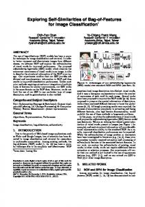
1. Introduction Figure 1. (a) An illustration of the distribution of local features and cluster centers by the K-means algorithm. (b) A demonstration of the relations among visual codes.

Automatic image classification is an important and challenging problem in computer vision. There are many solutions to this problem. Currently, one of the best image classification systems contains two key parts: the bag-offeatures (BOF) [7] model and the spatial pyramid matching (SPM) [11] technique. In the BOF model, an image is decomposed into a bag of local visual features which are described by a group of visual codes (codebook). After describing all features, all responses on each code are pooled over to one value by the maximum or the average operation. The image is finally represented by the responses of the codebook. The SPM technique partitions the image into spatial sub-regions, applies BOF on each sub-region and concatenates the histograms from all sub-regions. The BOF model plus the SPM technique achieves impressive performance on many databases, and plenty of extensions have been proposed.

In spite of these achievements, there is a common problem for the original BOF model and its extensions: each visual code is described by a single value after applying BOF. This strategy weakens codebook’s ability to describe images because each code has multiple aspects of properties. Figure 1(a) illustrates an example. The black points denote local features and the red triangles are clustering centers (visual codes) calculated by the k-means algorithm [16]. Every code occupies a region divided by the blue solid lines, each of which reflects one aspect of the code’s properties. In BOF, the response of each code is the number of points in its region. This scheme ignores the shape of the region 1649

supervised manner which maximizes the margin of local features from different categories [21],[6]. 3. Represent local features. This stage is also called ”coding” because local features are encoded by codes. There are some classic methods on this domain as follows.

determined by the blue solid lines. In fact, every blue solid line corresponds to a green dotted line in Figure 1(b) and indicates that two codes are related. This figure clearly shows that the codebook is not a set of discrete points but a graph, and a code’s properties are reflected by the relation between the code and its related neighbors. In this paper, we propose to model the relation of visual codes for image classification. In particular, we consider that the codebook is a graph, wherein a code is linked with a number of other codes. We employ the edges of the graph to reflect codes’ properties. This strategy contains much richer information of the codebook than the BOF model. Comprehensive experiments on the 15-Scenes and the Caltech101 databases demonstrate that considering code relation can stably and largely enhance the performance of various BOF based algorithms. In these two databases, our approach achieves very good performance comparable to the state-of-the-art algorithms. The rest of this paper is organized as follows. In Section 2, we introduce main components of the codebook based model. Section 3 explains our idea of exploring relations of visual codes, including constructing codebook graph and describing codebook graph. Section 4 provides experimental studies on the 15 natural scenes dataset and the Caltech101 database. Finally, we conclude the paper in Section 5.

• Hard voting [7]: Each local feature votes on its nearest code with one and other codes with zeros. This strategy may produce deviations, because most local features are just similar but not equivalent to codes. • Soft voting [17]: the soft voting scheme allows a local feature to vote on multiple related codes. It applies the distance between features and codes to calculate the probability that a feature belongs to a code. This approach preserves more information, i.e., similarity between codes and features, and achieves better performance than hard voting scheme. • Reconstruction based coding [20], [22], [19]: the sparse coding model [20] reconstructs a local feature using multiple codes via solving a leastsquare problem plus a L1 constraint to candidates. Afterwards, the sparse coding is extended to a more general framework: locally coordinate coding (LCC) [22]. This framework adds the constraint of local agglomeration of candidates. Yu et al. [22] proved that the local agglomeration constraint is beneficial for reducing representation deviation of local features. Recently, Wang et al. [19] proposed LCC’s fast version: locally linear coding (LLC) where the constraint of local agglomeration is replaced by searching K nearest candidates.

2. Related work In this section, we introduce the framework of the BOF model and discuss its various extensions. The BOF model consists of the following stages: 1. Extract local features for each image. The local features can be extracted from interesting areas via detectors or densely sampling. Classic detectors include Harris detector [10], maximally stable extremal region detector [13], affine invariant salient region detector [14], etc. Typical local descriptors include Haar descriptor [18], scale-invariant feature transform (SIFT) descriptor [12], gradient location and orientation histogram (GLOH) descriptor [15], shape context [5], histogram of oriented gradients (HOG) descriptor [8], etc. 2. Generate the codebook. Traditionally, the codebook is obtained via clustering over local features. The most widely used clustering algorithm is the k-means algorithm. It iterates the process that minimizes the sum of distance between clusters centers and data points, placing clusters near the most frequently occurring features. Recently, another scheme was proposed to produce the codebook, called dictionary learning. It includes two paradigms: unsupervised manner which repeatedly fits the codebook with local features [20], and

4. Pooling operation. After describing all local features, each code may obtain multiple responses. The pooling operation pools over these responses to one value. Classic pooling operations include max pooling and average pooling which preserve the max value and the average value from all responses respectively. In this paper, we focus on how to represent local features and generate responses on the codebook. The BOF model and its extensions use a single value for each code. This strategy weakens the ability of the codebook because they only reflect one aspect of each code. In the next section, we further discuss this problem and propose our solution.

3. Exploring relations among visual codes The BOF model borrows the idea from the bag-of-words (BOW) model applied for natural language processing and 1650

document classification. In BOW, sentences can be exactly represented by the frequency of each word because the set of words covers all possible components of a sentence or a paragraph. For image classification, however, the number of codes is much smaller than the number of possible local features1 . Most of features are similar but not equivalent to codes. Thus a feature can only describe one aspect of the code. For example, in Figure 2, the diamond feature is useful to reflect the relation between A and D but not the one between A and B.

||b − bn ||22 < λ||b − bN(1) ||22 ,

λ ∈ [1, ∞)

(3)

where N(i) is index of related neighbor of code b in the ith iteration; Δ(p1 , p2 , p2 ) denotes the angle decided by three points and p2 is the vertex; θ (domination region angle) and λ are two predefined parameters in the algorithm. Eq. (1) demands that the related neighbors are the nearest codes in the iteration. Eq. (2) indicates that the related neighbors should be not covered by existing domination regions. Eq. (3) requires the related neighbors be not far away from the code comparing with the nearest code. To intuitively understand the meaning of Eq. (1)∼(3), we take Figure 3 as an example. A, B, C, D are four codes. We explain how to obtain A’s related neighbors. Firstly, we find its nearest code B. Using A, B and the domination region angle θ, we get the first domination region Φ (A, B, θ). All other codes that located in this region, e.g., C, are not linked with A. In the second iteration, we find the nearest code D that satisfies two conditions:

Figure 2. An illustration showing that a feature can only reflect one aspect of a code’s properties.

The main claim in this paper is that the different properties of each code should be described respectively. This claim can be decomposed into two problems: 1) how many aspects of properties for each code; 2) how to describe each aspect. These two problems correspond to two stages in our method respectively: constructing the codebook graph and describing the codebook graph.

Δ(D, A, B) > θ

(4)

||A − D||22 < λ||A − B||22

(5)

Afterwards, a new domination region Φ (A, D, θ) is generated. We iterate this operation until all codes are considered.

3.1. Construct codebook graph To construct the codebook graph is to find each code’s related neighbors. We propose a domination region based algorithm to find the related neighbors for every code. The basic idea is that each related neighbor of a code is able to cover a region (domination region). Other codes in this region are suppressed, i.e., they do not link to this code. In detail, to obtain the index of a code b’s related neighbors N(i), we firstly find b’s nearest code bN(1) . Then we search other related neighbors by solving the following problem: N(i) = arg min ||b − bn ||22 , i ≥ 2

(1)

s.t. Δ(bn , b, bN(j) ) > θ, ∀j = 1, ..., i − 1

(2)

n

Figure 3. An illustration of codebook graph construction.

The domination region angle is an important parameter that affects the structure of the codebook graph. Figure 4 shows codebook graphs under different domination region angles. If the region angle is small, a code is linked with

1 For an image patch with the size of 16×16, the possible number of gray SIFT descriptors (8 directions) is 816×16 . But the number of codes is much less than a million.

1651

not Φ (A, B, θ). The BOF model does not distinguish these two different cases and thus loses useful information in describing codes. After all features are encoded, we obtain the responses of each code. In the BOF model, each code has one response, thus the final dimension of the histogram is four. In our method, we distinguish different properties of each code, and each code has multiple responses. The final dimension of the histogram is six.

many other codes. In the special case when the domination region angle is 0o , all codes are related each other. This means that each code is represented by M -1 values (M is the number of codes). As a result, a code has many domination regions, which may lead to the over-fitting effect. If the angle is large, a code is linked with a small number of neighbors and codes tend to be independent. Finally, we provide the pseudo-code of the algorithm in Algorithm 1. Input: B = [b1 , b2 , ..., bM ]: codebook Output: N = [N1 , N2 , ..., NM ], Nk is the index of the related neighbors of code bk . 1 foreach k = 1 : M do 2 i=2. 3 N1 (1) = the index of b1’s nearest code. 4 while do 5 Calculate Nk (i) using Eq. (1) ∼ Eq. (3). 6 if Nk (i) exists then 7 i=i+1; 8 end 9 else 10 break; 11 end 12 end 13 end Algorithm 1: Domination region based codebook graph construction

Figure 5. An demonstration of codebook description. Our method considers multiple properties of each code which are ignored by the BOF model

Next, we explain the motivation of each stage of the above process. 3.2.1

Searching code and domination region

Why should we consider only the nearest code and its nearest domination region in representing a feature? The Kmeans algorithm assigns a local feature to only one code because the optimization function of K-means algorithm is the sum of distance between cluster centers and data points:

3.2. Describe codebook graph arg min

The codebook is used to describe local features. In turn, the response of the codebook relies on local features2 . Thus, describing the codebook is transformed to representing features using the codebook. This process is divided into three stages: 1) searching each feature’s related domination region; 2) represent each feature in the domination region; 3) obtain the responses of each code from its domination regions. For a local feature, we first find its nearest code and all of this code’s domination regions, from which we choose the nearest domination region3 . Afterwards, we encode the local feature in this domination region. The responses of a code are generated in each of its domination region independently. Figure 5 illustrates an example. The diamond feature is used to reflect the domination region Φ (A, D, θ) but

  i

||ci − xj ||22

(6)

j∈S(ci )

where c and x denote clustering centers and data points respectively, and S(ci ) is the set of members belonging to cluster ci . The K-means algorithm tends to place clusters near the most frequently occurring features and assigns each feature to the nearest cluster center. Therefore, we consider that each local feature should only describe its nearest code. For simple and fast implementation, each local feature in our algorithm is used only once, so we search the nearest domination region of the nearest code. Further studies on searching multiple domination regions are meaningful, but we do not discuss them in this paper. 3.2.2

2 To describe a local feature, one or more codes will be used. As a result, these codes will generate responses on this local feature. 3 The distance between a point and a domination region is defined by the distance from the point to the angular bisector of the domination angle.

Representing local features

Our work can be considered as a framework. Various algorithms of representing local features can be embedded into 1652

Figure 4. Codebook graphs under different domination region angles. From left to right, the angles are 900 , 600 and 300 respectively. (λ = ∞)

Correspondingly, our method adds a code relation component to enhance the above two algorithms. They are:

our framework. Thus, the feature presentation is similar to previous algorithms, e.g., hard voting and sparse coding. The difference between our method and previous BOF models is that we use a sub-space (domination region) instead of the whole codebook space to describe each local feature. This is also convenient and unbiased for experimental comparison where all coding strategies are embedded into the same framework. 3.2.3

• Hard voting under average pooling operation plus code relation (HV+CR). • LLC under maximum pooling operation plus code relation (LLC+CR). The hard voting under average pooling operation is the most widely applied BOF model. It is the benchmark on many image classification databases. The LLC under maximum pooling operation is the very recently proposed coding strategy. The system based on this algorithm won PASCAL VOC 2009 on image classification. We comprehensively compare them with our algorithm in various cases. Since these algorithms are embedded into the same framework, the comparison among them is fair. In low level feature extraction, we use the gray SIFT descriptor [2] and dense sampling on a grid with step size of 4 pixels. The SIFT descriptor contains three scales: 16×16, 24×24 and 32×32. The K-means algorithm is used to generate the codebook and Lib-linear SVM [3] is employed for classification. The influence of other parameters will be discussed in the following experiments. All experiments are repeated ten times to obtain stable performance.

Obtaining responses of codes

In previous BOF models, the dimensionality of codebook representation is equal to the codebook size. This kind of representation can only reflect one aspect (or the average) of each code’s properties. In our approach, each code is reflected by multiple values, and the final dimensionality of codebook representation is the number of domination regions of all codes. Specifically, a pair of related codes, e.g., A and D in Figure 5, defines two domination regions: Φ (A, D, θ) and Φ (D, A, θ), corresponding to two dimensions of the codebook representation: AD and DA. Our codebook representation contains richer information of codes than the BOF model.

4. Experimental results

4.1. 15 natural scenes dataset

To demonstrate the effectiveness of our method, we evaluate it in two databases: the 15 natural scenes dataset [4] and the Caltech-101 databases [1]. As we analyzed before, our method is a general framework, any coding strategy and pooling operation can be embedded into it. Thus, we study our method using different coding schemes and pooling operation. In particular, we implement two baseline algorithms based on the BOF model:

There are 4,485 images in this dataset consisting of 15 kinds of natural scenes images. Each class contains at least 200 images. We employ the training and testing rule used by Lazebnik et al. [11]. That is, for each class, 100 images are randomly chosen as training samples and the rest are used for testing. On this dataset, we mainly study the influence of different parameters in our algorithm: the domination region angle θ in Eq. (2), the threshold λ in Eq. (3) and the codebook size. Table 1 and Table 2 show the performance of our

• Hard voting under average pooling operation (HV) [7]. • LLC under maximum pooling operation (LLC) [19]. 1653

79 classification accuracy

classification accuracy

78 77 76 75 74 73 72 71

HV HV + CR

70 64

128

256 512 1024 codebook size

2048

80 75 70 65 LLC LLC+CR

60

4096

64

128

(a) Using hard voting.

256 512 1024 codebook size

2048

4096

(b) Using LLC.

Figure 6. Performance comparisons among different methods on the 15 natural scene dataset.

method under different θ and λ. The codebook size is 4096. In this dataset, our approach performs best when θ = 90o and λ=1.5 although the difference is small. The experimental results also show that our algorithm is not sensitive to these two parameters. In the rest of the experiments, we fix θ to 90o and λ to 1.5.

hard voting drops a little but LLC can still be improved. We provide our understanding to this phenomenon. While, the maximum pooling operation preserves the distinctive representation to each local feature, hence a large number of codes can reflect many local features. The average pooling operation focuses on the global distribution of local features. What it needs is a suitable partition to the local feature space decided by the codebook size. If the codebook size is smaller or larger than the optimal value, the performance may decline.

Table 1. Performance of our approaches under different θ on the 15 natural scene dataset. (λ = 1.5) θ = 30o

θ = 60o

θ = 90o

θ = 120o

HV+CR

75.1±0.91

74.9±0.68

75.6±0.64

74.1±0.87

4.2. Caltech-101

LLC+CR

82.5±0.88

82.3±0.78

82.9±0.86

82.2±0.38

The Caltech-101 dataset contains 8,667 images, including101 object categories plus a background class. The number of images per class varies from 31 to 800. The images are with high shape variation, but objects are all centered and without viewpoint diversity. We use the common experimental rule on these two databases: for training, using different number of images; for testing, using at most 50 images per class. On this database, we study the influence of the codebook size to the performance of various algorithms under different number of training samples. The results are shown in Figure 7. The proposed code relation consistently enhances the performance of the baseline algorithms over all codebook sizes and numbers of training samples with a large margin. The best performance is achieved using LLC+CR when the codebook size is 8,192. In addition, we list some recently reported results on this database as well as our best performance in Table 3. Our result is competitive to the state-of-the-art performance on the Caltech-101 database.

Table 2. Performance of our method under different λ on the 15 natural scene dataset. (θ = 90o ) λ = 1.25

λ = 1.5

λ=2

λ = 2.5

HV+CR

75.5±1.21

75.5±0.23

74.5±0.41

73.1±0.91

LLC+CR

82.6±0.43

82.7±0.33

81.8±0.59

81.5±0.68

Figure 6(a) and Figure 6(b) show the performance of hard voting and LLC under various code sizes respectively. The results demonstrate that considering code relation can largely enhance the original algorithms. Besides, we note that hard voting outperforms LLC when the code size is small. However, as the codebook size increases, LLC is enhanced much faster than hard voting. When the code size comes to a relative high value, e.g., 512, the performance of 1654

Figure 7. Performance comparisons between HV, HV-CR, LLC and LLC-CR on the Caltech101 database under various codebook size and numbers of training samples. Table 3. Some excellent performance on the Caltech-101 database.

Training images

5

10

15

20

25

30

Lazebnik [11]

-

-

56.40

-

-

64.60

Yang [20]

-

-

67.00

-

-

73.20

Zhang [23]

46.60

55.80

59.10

62.00

-

66.20

Griffin [9]

44.20

54.50

59.00

63.30

65.80

67.60

Wang [19]

51.15

59.77

65.43

67.74

70.16

73.44

Ours

51.39

62.18

66.88

70.56

72.20

74.25

5. Conclusion

ture work. Finally, we conclude this paper with three main contributions of our work:

Previous BOF models ignore the relation among visual codes. In these algorithms, the codebook can be considered as a special graph which contains only notes but no edges. This graph can be generated by our method when the domination region angle θ is set to 360o . In this case, our approach is similar to common BOF models. Thus, we can consider that previous BOF models are special cases of our proposed framework. There are two factors that may affect the performance of our approach. The quality of the codebook graph partly depends on the distribution of visual codes. If the codebook unsuitably covers the local feature space, the generated graph cannot effectively describe images. In addition, to represent each local feature, we only use a simple strategy, i.e., search the nearest domination region to encode the feature. Other strategies are not studied in this paper. We believe that these factors are meaningful researches in fu-

1. Explain the BOF model in a novel viewpoint, i.e., a codebook is a graph in which the vertices (codes) are not independent. 2. Present a fast algorithm to construct the codebook graph and use it to describe images. 3. Largely improves the BOF model and its recent extensions in accuracy with slight additional computation cost.

Acknowledgement This work is supported by National Natural Science Foundation of China (Grant No.60875021,60723005), NLPR 2008NLPRZY-2, National Hi-Tech Research and 1655

Development Program of China (2009AA01Z318), Key Project of Tsinghua National Laboratory for Information Science and Technology.

[20] J. Yang, K. Yu, Y. Gong, and T. Huang. Linear spatial pyramid matching using sparse coding for image classification. CVPR, 2009. [21] J. Yang, K. Yu, and T. Huang. Supervised translationinvariant sparse coding. CVPR, 2010. [22] K. Yu, T. Wang, and Y. Gong. Nonlinear learning using local coordinate coding. NIPS, 2009. [23] H. Zhang, A. Berg, M. Maire, and J. Malik. Svm-knn: Discriminative nearest heighbor classification for visual category recognition. CVPR, 2006.

References [1] www.vision.caltech.edu/Image_Datasets/ Caltech101/. [2] http://www.vlfeat.org/. [3] http://www.csie.ntu.edu.tw/˜cjlin/ liblinear/. [4] http://www.cs.unc.edu/˜lazebnik/ research/scene_categories.zip/. [5] S. Belongie, J. Malik, and J. Puzicha. Shape matching and object recognition using shape contexts. IEEE Trans. on Pattern Analysis and Machine Intelligence, 24(4):509–522, 2002. [6] D. M. Bradley and J. A. Bagnell. Differential sparse coding. NIPS, 2008. [7] G. Csurka, C. Bray, C. Dance, and L. Fan. Visual categorization with bags of keypoints. ECCV, 2004. [8] N. Dalal and B. Triggs. Histograms of oriented gradients for human detection. CVPR, 2005. [9] G. Griffin, A. Holub, and P. Perona. Caltech-256 object category dataset, 2007. [10] C. Harris and M. Stephens. A combined corner and edge detector. Proceedings of the Fourth Alvey Vision Conference, pages 147–151, 1988. [11] S. Lazebnik, C. Schmid, and J. Ponce. Beyond bags of features: Spatial pyramid matching for recognizing natural scene categories. CVPR, 2006. [12] D. G. Lowe. Distinctive image features from dcale-invariant key-points. International Journal of Computer Vision, 2(60):91–110, 2004. [13] J. Matas, O. Chum, M. Urban, and T. Pajdla. Robust widebaseline stereo from maximally stable extremal regions. Image and Vision Computing, 22(10):761–767, 2004. [14] K. Mikolajczyk and C. Schmid. Scale and affine invariant interest point detectors. International Journal of Computer Vision, 60(1):63–86, 2004. [15] K. Mikolajczyk and C. Schmid. A performance evaluation of local descriptors. IEEE Trans. on Pattern Analysis and Machine Intelligence, 27(10):1615–1630, 2005. [16] S.P.Lloyd. Least squares quantization in pcm. IEEE Transactions on Information Theory, 28(2):129–137, 1982. [17] J. van Gemert, J. Geusebroek, C. Veenman, and A. Smeulders. Kernel codebooks for scene categorization. ECCV, 2008. [18] P. Viola and M. Jones. Robust real-time object detection. Proc. of IEEE Workshop on Statistical and Computa-tional Theories of Vision, 2001. [19] J. Wang, J. Yang, K. Yu, F. Lv, T. Huang, and Y. Gong. Locality-constrained linear coding for image classification. CVPR, 2010.

1656