Exposure at Default models with and without the Credit Conversion Factor Edward Tong, Christophe Mues, Iain Brown, Lyn Thomas
[email protected] Credit Scoring and Credit Control XIV Edinburgh, August 26-28 2015
Disclaimer
The opinions expressed in this document are solely the authors’ and do not necessarily reflect those of the Bank of America or any of its subsidiaries.
2
EAD (Exposure at Default) Basel II/III - requirement for Internal Ratings Based (IRB) Advanced approach for calculating minimum capital requirements, CCAR stress testing EAD defined as gross exposure in the event of obligor default, typically in 12 months This study: EAD for credit cards (revolving exposures) 3
EAD model approaches Notation E(td) = EAD E(tr) = balance at time r L(tr) = limit at time r
Credit limit (£) Undrawn amount
EAD12 months
Undrawn amount × CCF12 months
Drawn amount
Drawn amount
12 months
Issued credit
Time
t0
Credit conversion factor (Taplin et al. 2007, Jacobs 2010, Qi 2009) CCF
E td E t r L tr E t r
EAD Current Drawn CCF Current Undrawn
4
EAD model approaches (cont’d) Notation E(td) = EAD E(tr) = balance at time r L(tr) = limit at time r
Utilization change (Yang & Tkachenko, 2012) utilch
E td E tr L tr
Direct EAD based on OLS (Taplin et al., 2007) Mixture models (Witzany, 2011, Leow & Crook, 2013) 5
Research objectives To directly model the EAD amount Compare performance of direct EAD models with known industry models – Credit Conversion Factor (CCF) and Utilization Change Consider segmentation by credit usage to combine direct EAD and CCF models
Model time to default as a predictive variable using weighted PD approach
6
Data UK bank Credit card portfolio 3 years of data (2001 to 2004) All observations are defaulted accounts >10k defaults in total sample
7
Data (cont’d) Response variables of EAD, CCF, Utilization Change
11 behavioural variables including Committed Size / Amount Drawn, Undrawn Amount Drawn Percentage (Credit Usage) Time to Default Rating Class Average Days Delinquent Absolute Change in Drawn Amount
8
Response variables EAD and CCF
9
Fitted EAD distribution Training set
10
Zero-adjusted gamma distribution The probability function of the ZAGA is defined by
if y 0 1 y 12 1ey 2 fY y | , , 1 2 1 2 1 2 if y 0 for 0 y < , 0 < < 1, 0, 0 where denotes mean, scale, probability of zero EAD
E Y 1 and Var Y 1 2 2
11
Generalized Additive Model for Location, Scale & Shape GAMLSS (Rigby & Stasinopoulos, 2005, 2007, 2015) implemented in gamlss package in R General framework for regression models Response variable y ~ D(y | µ, σ, ν, τ) where D() can be any distribution (over 70 different types including highly skew and kurtotic distributions) Mortgage LGD model (Tong et al., 2013)
12
ZAGA model setup J1
log 1 11 h j1 x j1 j 1
J2
log 2 22 h j 2 x j 2 j 1
J3
logit 3 33 h j 3 x j 3 j 1
where k k denote parametric linear terms,
h jk x jk denote additive smoothers
13
ZAGA model development Separate model components estimated for µ, σ and π components
Developed with stepwise selection based on Akaike Information Criteria (AIC) Continuous variables fitted with smoothers based on penalized B-splines (Eilers & Marx, 1996) 14
Results Mean of non-zero EAD
15
Results Dispersion of non-zero EAD
Dispersion increases with Undrawn (%), decreases with credit usage
16
Benchmark models: CCF, Util. Change, PD weighted 3 CCF models based on OLS, Fractional Response Regression (Papke & Woolridge, 1996) and Tobit models (Tobin, 1956) Utilization Change based on Tobit model Survival EAD model - PD weighted approach to model time to default using Cox PH regression: S t 1 S t EAD EAD t 1 S (t 12) t 1 12
17
Benchmark models: Segmentation by credit usage Segmentation using combined Direct EAD (ZAGA) and CCF models
CCF models perform better for low credit usage, Direct EAD model better for high credit usage Credit usage of 90% was optimal cut-off for segmentation based on discrimination and calibration performance measures 18
Validation methodology 10-fold cross validation (CV) Spearman ρ MAE from EAD MAEnorm from
EAD Commitment Size
RMSE, RMSEnorm 19
Validation with 10 fold CV OLSCCF
TobitCCF
FRRCCF
TobitUTIL
OLSEAD
ZAGAEAD
OLSUSE
ZAGAUSE
Spearman ρ
0.741
0.737
0.743
0.746
0.744
0.742
0.750
0.749
MAE
859.0
870.6
856.1
925.2
883.3
833.5
829.9
819.2
RMSE
1614.8 1586.3 1577.7 1654.3
1546.1 1602.5
1565.7 1571.0
MAEnorm
0.273
0.276
0.273
0.294
0.301
0.268
0.269
0.260
RMSEnorm
0.432
0.430
0.430
0.442
0.448
0.454
0.430
0.429
ZAGA-EAD, ZAGA-USE have lowest MAE Survival EAD MAE=830.3, MAEnorm=0.266
20
Validation Observed vs Fitted EAD Densities
21
Conclusions Modelling the EAD amount directly can produce competitively predictive EAD models Segmentation by credit utilization offers greater performance benefits - a combined approach with EAD and CCF models may work better The time to default variable can be used a priori within a PD weighted model
22
References Djennad, A.D., Rigby R., Stasinopoulos, D., Voudouris, V., Eilers, P.H.C. (2015). Beyond location and dispersion models: the Generalized Structural Time Series Model with Applications. http://papers.ssrn.com/sol3/papers.cfm?abstract_id=2577330 Eilers, P. H. C., & Marx, B. D. (1996). Flexible smoothing with B-splines and penalties. Statistical Science, 11(2), 89-102. Jacobs, M., Jr. (2010). An Empirical Study of Exposure at Default. Journal of Advanced Studies in Finance, 1, 31-59. Leow, M., Crook, J. (2013). A Two Stage Mixture Model for Predicting EAD. Credit Scoring & Credit Control XIII. Edinburgh, UK.
Qi, M. (2009). Exposure at Default of Unsecured Credit Cards. Economics Working Paper 2009-2. Office of the Comptroller of the Currency. Rigby, R. A. and Stasinopoulos D. M. (2005). Generalized Additive Models for Location, Scale and Shape. Applied Statistics, 54, 507-554. Rigby, R. A. & Stasinopoulos, D. M. (2007). Generalized Additive Models for Location Scale and Shape (GAMLSS) in R. Journal of Statistical Software, 23. Taplin, R., Minh To, H. & Hee, J. 2007. Modeling exposure at default, credit conversion factors and the Basel II Accord. The Journal of Credit Risk, 3, 75-84. Tong, E. N. C., Mues, C. & Thomas, L. (2013). A zero-adjusted gamma model for mortgage loan loss given default. International Journal of Forecasting, 29, 548-562. Yang, B. H. & Tkachenko, M. 2012. Modeling exposure at default and loss given default: empirical approaches and technical implementation. The Journal of Credit Risk, 8, 81-102. Witzany, J. 2011. Exposure at Default Modeling with Default Intensities. European Financial and Accounting Journal, 6, 20-48.
23