FUZZ-IEEE 2009, Korea, August 20-24, 2009
Extended T-S Fuzzy Model based on Interval Arithmetic and Its Application to Interval Nonlinear Regression Analysis Sun Changping and Xu Zhengguang, Member, IEEE
Abstract—In this paper, a new fuzzy system model structure –Interval T-S Fuzzy Model (ITSFM) is proposed. Inspired from interval regression analysis, the interval arithmetic is incorporated with classical T-S fuzzy model and the parameters in consequent part of the ITSFM model become to be interval numbers. Thus, the outputs of the proposed ITSFM are interval numbers. In our ITSFM model, the membership functions are the same as the ones of the classical type. Finally, the proposed ITSFM is applied to interval nonlinear regression analysis with crisp inputs and interval outputs. Experimental results are then presented that indicate the validity and applicability of the proposed ITSFM.
I. INTRODUCTION
C
lassical fuzzy logic systems (FLS) are able to construct a nonlinear relation for crisp input and output data. It has been used in many fields, such as system identification [1], fuzzy control [13], and fault detection [14]. However, in practical applications, the available information is often uncertain, imprecise and incomplete. Interval-valued data offer a valuable way of representing the available information in complex problems where imprecision or variability must be taken into account. Nevertheless, the classical fuzzy logic (FL) cannot fully handle all the uncertainty present in real-world problems [12]. In order to handle the uncertainty, the type-2 fuzzy logic systems (FLS) were proposed in recent years [7]. It translate all the uncertainties of the measurement into uncertainties about the membership functions, and results in a notation that gives the third dimension to the membership functions of the classical type. Nevertheless, most general type-2 FLS are rather computation intensive. Interval type-2 FLS are later used to simplify computation by identifying the foot print of uncertainty of fuzzy sets [8]. Comparing with classical fuzzy logic systems, the computation of interval type-2 FLS is still large. In [5], a probabilistic fuzzy logic system (PFLS) was proposed for modeling a system with stochastic uncertainties. Different to the ordinary FLS, the PFLS uses the probabilistic fuzzy set instead of the ordinary fuzzy set. Thus it is able to capture the information with stochastic uncertainties. But in practical applications, it is hard to determine probabilistic density function of fuzzy membership grade. Both type-2 FLS and PFLS capture the uncertainties in the system by adding This work was supported by the Key Disciplines Construction Project of Beijing under Grant XK100080537. The authors are with the Key Laboratory of Advanced Control for Iron and Steel Process(University of Scinece and Technology Beijing), Ministry of Education, University of Science and Technology Beijing, China. (e-mail:
[email protected];
[email protected]) . 978-1-4244-3597-5/09/$25.00 ©2009 IEEE
additional information to membership functions of the classical type to form a generalization membership functions. In [11], an interval fuzzy modeling method was proposed. It results in lower and upper fuzzy models with a set of lower and upper parameters by the min–max optimization method. However, the approaches described above are only can be used to construct a nonlinear relation for crisp input and output data in the framework of fuzzy systems. In other words, those approaches have incapability of modeling with crisp inputs and interval outputs. Fuzzy regression analysis introduced by Tanaka etal is another approach to dealing with uncertainty information [6]. Interval regression analysis, where a model with interval coefficients is assumed, is regarded as the simplest version of fuzzy regression analyses [4]. In order to endow the classical T-S fuzzy model with the ability of constructing a model with crisp input and interval output data, in this paper, an extended T-S fuzzy model–Interval T-S Fuzzy Model (ITSFM) is proposed. Different to the existing approaches handling with the uncertainties in the system by adding additional information to membership functions of the classical type to form a generalization membership functions, in our ITSFM model, the interval arithmetic is incorporated with classical T-S fuzzy model and the parameters in consequent part of the ITSFM model become to be interval numbers. Thus, the uncertainty of available information is characterized by the interval consequent parameters of the ITSFM. However, the membership functions in the proposed fuzzy model are still the same as the ones of the classical type. Finally, the proposed ITSFM is applied to interval regression analysis with crisp inputs and interval outputs. The simulation results show that the proposed ITSFM can achieve a better modeling performance for interval regression analysis. This paper is organized as follows: In SectionⅡ, we brief review of the theory of interval arithmetic and interval regression; the ITSFM model based on interval arithmetic is introduced, then the formulations of interval regression based on ITSFM is deduced in Section Ⅲ ; Section Ⅳ , the experiments are presented. Finally, the conclusion is gives in SectionⅤ. II. SOME RESULTS IN INTERVAL ARITHMETIC AND INTERVAL REGRESSION ANALYSIS In this section, we need to briefly look at some important formulations in interval arithmetic and interval regression analysis [2], [9].
1773
FUZZ-IEEE 2009, Korea, August 20-24, 2009
A. Interval arithmetic An interval number can be represented by its lower and upper limits as A = [a L , aU ] , or, equivalently, by its midpoint
and radius as A = (ai , ci ) , where a C = (a L + aU ) / 2
Y∗ (xi ) = ( a t t
(1)
A - B = [ a L − bU , aU − b L ]
(2)
λ ⋅ A = [λ ⋅ a L , λ ⋅ aU ] where λ is a constant and λ >0.
(3)
n
min J P = ∑ (c t | x i | +d t | x i | ) : Possibility model
C
R
R
A +B =(a +b ,a +b )
(4)
A - B = ( a C − bC , a R + b R )
(5)
C
R
λ ⋅ A = (λ ⋅ a , λ ⋅ a )
(6)
B. Interval regression analysis based on possibility and necessity models In this section, we review unified QP approach [2] to obtain the possibility and necessity models simultaneously. In this unified approach, we assume for simplicity that the center coefficients of the possibility regression model and necessity regression model are same. Assume that input and output data are given as ( x i ; Yi ) =
(11)
i =1
n
max J N = ∑ c t | x i | : Necessity model.
(12)
i =1
The objective function of the unified model can be obtained by the combination of these two objective functions. The combination of two functions yields the following: n
If the interval number A and B are represented by its midpoint and radius, the operations defined on the interval numbers are respectively C
(10) t
where a = ( a0 , a1,…, am ) , c = ( c0 , c1 ,…, cm ) The two objective functions in the possibility and necessity models are assumed as follows:
and a R = (aU − a L ) / 2 . Let A and B be two intervals represented by its lower and upper limits, the operations defined on the interval numbers are, respectively.
A + B = [ a L + b L , aU + bU ]
xi , c t | xi | )
Min J P − J N = ∑ dt | xi |
(13)
i =1
Then, the objective function in the unified approach by QP can be assumed as the following quadratic function: n
n
i =1
i =1
J = ∑ (d t | x i |) 2 = dt (∑ | xi | | xi |t )d
(14)
Therefore interval regression analysis is to determine the interval coefficients Ai∗ and A∗i , i = 0,1,… , m that minimize the aforementioned objective function J and satisfy inclusion relations Y∗ ( X i ) ⊆ Yi ⊆ Y ∗ ( X i ) . This can be described as the following QP problem: n
min J = d (∑ | xi | | xi | )d + ξ ( at a + c t c ) t
t
i =1
Y ∗ (xi ) = A0∗ + A1∗ xi1 + … + Am∗ xim ,
i = 1, … , n
(7)
⎧a t x i + c t | x i | +d t | xi |≥ yi + ei ⎪ ⎪a t x i − ct | x i | −d t | x i |≤ yi − ei ⎪⎪ subject to ⎨a t x i + c t | x |≤ yi + ei (15) ⎪ t t i = 1, … , n ⎪a x i − c | x |≥ yi − ei ⎪ ci ≥ 0, d i ≥ 0 i = 0,1, … , n ⎪⎩ where ξ is a significantly small positive number, and so leads
Y∗ (xi ) = A∗ 0 + A∗1xi1 + … + A∗ m xim ,
i = 1, … , n
(8)
the influence of ξ ( at a + c t c ) to be negligible.
(1, xi1 , … , xim ; Yi ), i = 1,…, n where x i is the ith input vector, Yi is the corresponding interval output that consists of a center y i and a radius ei denoted as Yi = ( y i , ei ) , and n is a data size. For this data set, the possibility and necessity estimation models are denoted as
where the interval coefficients Ai∗ and A∗i are denoted as Ai∗ = ( ai∗ , ci∗ ) and A∗i = (a ∗i , c ∗i ) , respectively. The estimated interval Y ∗ (xi ) by the possibility model always includes the observed Yi , whereas the estimated interval Y∗ (xi ) by the necessity model should be included in the observed interval Yi . In fact, we can denote the interval coefficients Ai∗ and A∗i as Ai∗ =( ai , ci + di )
A∗i =( ai , ci )
which satisfies the condition A∗i ⊆ Ai∗ , i = 0,1,… , m since c i and d i are assumed to be nonnegative. Therefore, from formulations (4) and (6), the possibility model Y ∗ (xi ) and the necessity model Y∗ (xi ) can be written as Y ∗ (xi ) = ( a t
xi , c t | xi |+ d t | xi | )
(9)
III. INTERVAL T-S FUZZY MODEL AND ITS APPLICATIONS TO INTERVAL REGRESSION Classical T-S model is able to construct a nonlinear relation for crisp input and output data. However, to the best of our knowledge, there is no fuzzy system model structure being able to construct a nonlinear relation for crisp input and interval output data directly. In order to overcome the above shortcoming of classical fuzzy system model structure, we introduce interval arithmetic to classical T-S fuzzy model. Before introducing the proposed ITSFM, we first review the classical T-S fuzzy model. A. Classical T-S fuzzy model T-S fuzzy model deals with a complex system by decomposing input space into several subspaces, each of which is represented by a simple linear model. Generally, its rules take on the following form [10]:
1774
FUZZ-IEEE 2009, Korea, August 20-24, 2009
R i : If x1 is A1i and x 2 is A2i ,…, x n is Ani
Then h i = f i ( x1 , x 2 ,
r
~ [(a i , c i ) + (a i , c i ) x + =∑w 0 0 1 1 1 i
, x n ) = α 0i + α 1i x1 +
+ α ni x n = α ti x , (16) For i = 1,2, … , r , where r denotes the number of rules, A ij is
i =1
yˆ (x) =
∑ wi hi i =1 r
∑w
i
r
r
i =1
i =1
~ hi = w =∑w ∑ ~i α ti x i
∏
i =1
i =1
where A i = (a 0i , a1i ,
, a ni ) t , C i = (c 0i , c1i ,
, c ni ) t , , xn ) t
Yˆ (x) = ( A t ~ x, C t ~ x)
i ~ = w Aij ( x j ) , and w i r j =1 ∑ wi
B. The proposed Interval T-S fuzzy model (ITSFM) The proposed ITSFM has the same model structure as classical T-S fuzzy model except that the parameters in consequent part of the ITSFM model become to be interval numbers. Thus, the outputs of the proposed ITSFM are interval numbers. The proposed ITSFM consists of a set of IF-THEN rules with the form: R i : If x1 is A1i and x 2 is A2i ,…, x n is Ani (18)
( A1t , A t2 ,
, A tr ) t
(21)
i =1
(22)
A= , C= , C tr ) t ~ x t,w ~ x t, ,w ~ x t )t , ~ xt , w ~ xt , w ~ xt )t , ~ x = (w x = (w ,~ r 1 2 1 2 r t~ t ~ A x and C x are the center and radius of the predicted
n
+ θ ni x n = θ ti x ,
r
∑ w~i C ti x )
x = (1, x1 , x 2 , , x n ) t , x = (1, x1 , x 2 , Furthermore, Yˆ (x) can be expressed as
where
i =1
Then Y i = θ 0i + θ 1i x1 +
r
(17)
i =1
where the weight w i =
r
~ ( A t x, C t x ) = ( w Yˆ (x) = ∑ w ∑ ~i A ti x, i i i
t
r
(20)
~ ≥ 0 , one obtains: From formula (4), (6) and w i
the corresponding fuzzy set, and α i = (α 0i , α 1i , … , α ni ) t is the parameter set in the consequent part, x = [1, x1 , x2 , , xn ] is a real input vector. The predicted output of the fuzzy model is inferred as
+ (a ni , c ni ) x n ]
(C1t , C t2 ,
interval output Yˆ (x) , respectively. Algotithm: Interval T-S fuzzy modeling for crisp inputs and interval outputs. Inputs: Crisp data x j =( x j1 , … , x jn ) t Outputs: Interval data Y j =( y j , e j ), j = 1, … , p , y j and e j are the center and radius of interval number Y j , respectively. Step 1: The fuzzy partition of input variables, obtain the fuzzy membership functions Aij ( x j ) , for example by Fuzzy
consequent part of the ITSFM, θ ij = (a ij , c ij ) is an interval
C-means algorithm. Step 2: Computing the interval output of ith rule based on interval arithmetic. Step 3: Computing the final interval outputs of the ITSFM by formula (19). Step 4: Estimate the consequent interval parameters θ i = (θ 0i , θ1i , θ ni ) t , for example by LSM. That is, A can be
number, a ij and c ij are the center and radius of θ ij ,
obtained by min
Y i is the interval output of ith rule, i = 1, 2, … , r , where
r denotes the number of rules, x = (1, x1 , x 2 ,
x n ) t is the
real-valued input vector, A ij is the corresponding fuzzy set, θ i = (θ 0i , θ1i ,
θ ni ) t is the interval parameter vector in the
p
respectively, j = 0,1, … , n . The predicted interval output of the ITSFM, that is, Yˆ (x) is inferred as
j =1
p
∑ (e j − | Ct ~x j |) 2 .
r
Yˆ (x) =
∑ wi i =1
where w = ∏ i
n Ai ( x j ) j =1 j
i ~ = w , then Yˆ (x) can be expressed as Let w i r ∑ wi i =1
r
~Yi Yˆ (x) = ∑ w i
j =1
∑ wiY i i =1 r
∑ ( y j − A~x j ) 2 , C can be obtained by min
(19)
C. Interval nonlinear regression analysis based on ITSFM Classical T-S model is able to construct a nonlinear relation for crisp input and output data. Likewise, the ITSFM can construct a nonlinear mapping with crisp inputs and interval outputs. In the framework of the ITSFM, the possibility model and the necessity model [2] are combined with the ITSFM, then the interval nonlinear regression formulations are presented. In the framework of the ITSFM, the possibility model Yˆ ∗ (x i ) and the necessity model Yˆ∗ (x i ) can be written as: r
i =1
~ θ∗t x Yˆ ∗ (x) = ∑ w i i
r
~ θt x =∑w i i
i =1
i =1
1775
(23)
FUZZ-IEEE 2009, Korea, August 20-24, 2009 r
~ θt x Yˆ∗ (x) = ∑ w i ∗i where θ∗i = (θ 0∗i , θ1∗i ,
i =1 ∗i t θn ) ,
(24)
θ ∗j i = (a ij , c ij + d ij ) ,
, θ ∗i n ) t , θ ∗i j = (a ij , c ij ) , c ij ≥ 0 , d ij ≥ 0 ,
θ∗i = (θ ∗i0 , θ ∗i1 ,
i = 1, 2, … , r , j = 0,1, … , n
From formula (20), (21), (22), expressed as Yˆ ∗ (x) =( A t ~ x, C t ~ x + Dt Yˆ (x) = ( A t ~ x, C t ~ x ),
Yˆ ∗ (xi ) , Yˆ∗ (x) can be ~ x ),
(25) (26)
∗
where D = (D1t , D t2 , , D tr ) t , D ti = ( d 0i , d1i , d ni ) , i = 1, 2, … , r Suppose that we are given the training data ( x j ; Y j ) = (1, x j1 , … , x jn ; Y j ), j = 1, … , p where
x j is the jth input
vector, Y j is the corresponding interval output that consists of a center y j and a radius e j denoted as Y j = ( y j , e j ) , and
p is a data size. In the framework of the ITSFM, interval nonlinear regression analysis based on the possibility model and the necessity model can be resolved by solving the following QP problem:
We now adopt the measure of fitness (for details, see [2] ) to compare the proposed method with the methods of Tanaka’s [2] and Hong’s [3]. In the case of the linear model , the measure of fitness for ith data ϕ Y (x i ) is defined as c t | x i | +d t | x i | which indicates how closely the possibility output for the ith input approximates the necessity output for the ith input. Here, the denominator and the numerator represent the spreads of the estimated intervals Yˆ ∗ (x) and Yˆ∗ (x) , respectively. Then , the measure of fitness for all data defined as ct | x j | 1 p 1 p ϕY = ∑ ϕ Y ( x j ) = ∑ t p j =1 p j =1 c | x j | +d t | x j |
also define ϕ Y (x i ) and
ϕ Y for nonlinear model by using the
ϕY (x j ) is defined as
j =1
TABLE Ⅱ OBTAINED ϕY ( x j ) AND
| +D | ~ x j |≥ y j + e j t ~ | − D | x j |≤ y j − e j t
No.(i)
|≤ y j + e j |≥ y j − e j
j = 1, …, p
i = 1, …, r , l = 0,1, …, n (27)
where ξ is a significantly small positive number.
is
corresponding spreads of the estimated intervals Yˆ ∗ (x) and Yˆ∗ (x) . In this paper, the measure of fitness for jth data
min J = D (∑ | ~ xj || ~ x j |t ) D + ξ ( A t A + C t C )
⎧A t ~ x j + Ct | ~ xj ⎪ t t ~ ~ ⎪A x j − C | x j ⎪ ⎪ subject to ⎨ A t ~ x j + Ct | ~x j ⎪ t~ t ~ ⎪A x j − C | x j ⎪ i i ⎪⎩ cl ≥ 0, d l ≥ 0
ϕY
where p is a sample size and 0 ≤ ϕY ≤ 1. The larger the value of ϕY , the better the model is fitting the data. We can
p
t
ct | xi |
ϕY (x i ) =
IV. NUMERICAL EXAMPLE In this section, we use one data set, crisp inputs-interval outputs shown in TableⅠ. This data is taken from Tanaka and Lee [2]. The proposed ITSFM is applied to this data set from an illustrate point of view. We use fuzzy c-means clustering algorithm to find the parameters in premise part of the ITSFM. Fig.1-Fig.3 illustrate the results for the proposed ITSFM with clustering number r is 2, 3, 4 , respectively . In each figure, the outer two lines represent the possibility model Yˆ ∗ (x) and the inner two lines represent the necessity model Yˆ (x) . From Fig.1-Fig.3 we realize the proposed ∗
ITSFM performs very well. TABLE Ⅰ CRISP INPUT-INTERVAL OUTPUT DATA No.
1
2
3
4
5
6
7
8
x
1
2
3
4
5
6
7
8
Y
[15,30]
[20,37.5]
[15,35]
[25,60]
[25,55]
[40,65]
[55,95]
[70,100]
1776
ϕY
Model:
FOR NUMERICAL DATA
ϕY (x j )
1 2 3 4 5 6 7 8
Tanaka’s 0.1277 0.1591 0.1826 0.2008 0.2153 0.2271 0.2369 0.2452
Hong’s 0.7201 0.2397 0.2736 0.4969 0.6695 0.7158 0.6943 0.8004
ITSFM’s (r=4) 0.9803 0.9447 0.7509 0.7465 0.8350 0.8365 0.7397 0.7316
ITSFM’s (r=3) 0.2452 0.1722 0.3731 0.6461 0.6605 0.6608 0.7212 0.7088
ϕY
0.1994
0.5763
0.8206
0.5235
ϕY (x j ) =
Ct | ~ xj | t ~ C | x j | +Dt | ~ xj |
Then , the measure of fitness for all data ϕ Y is defined as Ct | ~ xj | 1 p ϕY = ∑ t ~ p j =1 C | x j | + D t | ~ xj |
FUZZ-IEEE 2009, Korea, August 20-24, 2009
clustering number 3 are near to those of Hong’s , but is much larger than those in quadratic model of Tanaka’s . When clustering number r=4, the values of ϕY ( x j ) and
120
100
ϕY in the proposed ITSFM are much larger than those in quadratic model of Tanaka’s and in SVM nonlinear model of Hong’s, respectively. Thus, the measure of fitness indicates that the ITSFM is providing the best fit to the given data compared to the other models.
Interval output Y
80
60
40
V. CONCLUSION
20
0
0
1
2
3
4 5 Crisp input x
6
7
8
In this paper, a new fuzzy system model structure –Interval T-S Fuzzy Model (ITSFM) is proposed. It extends the parameters in consequent part of classical T-S fuzzy model to be interval numbers, thus the uncertainty of available information is characterized by the interval-valued consequent parameters of the ITSFM. Therefore the proposed ITSFM have capability of modeling with crisp inputs and interval outputs. The application of the proposed ITSFM to nonlinear regression analysis with crisp inputs and interval outputs verifies the validity and applicability of the proposed ITSFM. In the future, we believe that the ITSFM will be very promising for many engineering applications, such as system identification, robust control and decision making [15], etc., where the available uncertain information is represented by interval number.
9
Fig. 1. Obtain interval nonlinear model by the proposed ITSFM (clustering number r is 2) 110 100 90
Interval output Y
80 70 60 50 40 30 20
0
1
2
3
4 5 Crisp input x
6
7
8
9
Fig. 2. Obtain interval nonlinear model by the proposed ITSFM (clustering number r is 3) 110 100 90 80 Interval output Y
REFERENCE A. Ernesto and D. S. C. Leandro, “Fuzzy model and particle swarm optimization for nonlinear identification of a Chua's oscillator,” in Proc.16th IEEE Int. Conf. Fuzzy Syst., London, UK, Jul. 2007, p4295644 [2] H. Tanaka and H. Lee, “Interval regression analysis by quadratic programming approach,” IEEE Trans.Fuzzy Systems, vol.6, pp. 473-481, November 1998 [3] D. H. Hong and C. H. Hwang, “Interval regression analysis using quadratic loss support vector machine,” IEEE Trans.Fuzzy Systems, vol.13, pp. 229-237, April 2005.. [4] C. H. Hwang, D. H. Hong, and K. H. Seok, “Support vector interval regression machine for crisp input and output data,” Fuzzy Sets Syst, vol.157, pp. 1114-1125, 2006 [5] Z. Liu and H. X. Li, “A probabilistic fuzzy logic system for modeling and control,” IEEE Trans. Neural Networks, vol. 13, pp. 848–859, December 2005 [6] H. Tanaka, S.Uejima, and K. Asai, “Linear regression analysis with fuzzy model,” IEEE Trans. Syst., Man, Cybern., vol. 12, pp. 903-907,1982 [7] N. N. Karnik, J. M. Mendel and Q. L. Liang, “Type-2 fuzzy logic system,” IEEE Trans.Fuzzy Systems, vol.7, pp. 643-658, December 1999 [8] Q. L. Liang and J. M. Mendel, “Interval type-2 fuzzy logic systems: theory and design,” IEEE Trans.Fuzzy Systems, vol.8, pp. 535-550, October 2000. [9] R. E. Moore, Interval analysis. Prentice-Hall: Englewood Cliffs, NJ, 1966. [10] T. Takagi, M.Sugeno, Fuzzy identification of systems and applications to modeling and control, IEEE Trans. Syst. Man Cybern, vol. 15, pp. 116-132, January 1985.. [11] I. Skrjanc, S. Blazic and O. Agamennoni, “Interval fuzzy model identification using l ∞ -norm,” IEEE Trans.Fuzzy Systems, vol.13, pp. [1]
10
70 60 50 40 30 20 10
0
1
2
3
4 5 Crisp input x
6
7
8
9
Fig. 3. Obtain interval nonlinear model by the proposed ITSFM (clustering number r is 4)
Table Ⅱ shows the obtained ϕ Y (x j ) and ϕY for the quadratic model of Tanaka’s, the nonlinear model of Hong’s, and the proposed ITSFM. In the proposed ITSFM, the fuzzy rule number is 3, 4, respectively, and the membership degree is determined by fuzzy c-means clustering algorithm. From Table Ⅱ, we can observe that the values of ϕY ( x j ) and ϕY in the proposed ITSFM with
561-568, October 2005 [12] J. M. Mendel, Uncertain rule-based fuzzy logic systems, introduction and new directions, Prentice Hall, 2001.
1777
FUZZ-IEEE 2009, Korea, August 20-24, 2009
[13] W. Xie, “Improved L2 gain performance controller synthesis for Takagi-Sugeno fuzzy system,” IEEE Trans.Fuzzy Systems, vol.16, pp. 1142-1150, October 2008. [14] F. J. Uppal and R. J. Patton, “Neuro-fuzzy uncertainty de-coupling: a multiple-model paradigm for fault detection and isolation,” Int. J. Adapt. Control Signal Process, vol.19, pp.281-304, May 2005 [15] R. R. Yager, “Fuzzy modeling for intelligent decision making under uncertainty,” IEEE Trans. Syst., Man,Cybern. B, Cybern,vol.30, no.1, pp. 60-70, January 2000.
1778