Extracting Complex Dielectric Properties from ...

This article has been accepted for publication in a future issue of this journal, but has not been fully edited. Content may change prior to final publication. Citation information: DOI 10.1109/ACCESS.2018.2797698, IEEE Access

1

Extracting Complex Dielectric Properties from Reflection-Transmission Mode Spectroscopy Jingye Sun and Stepan Lucyszyn, Fellow, IEEE

Abstract — Material characterization of homogeneous dielectric slabs using reflection-transmission mode spectroscopy can be problematic due to the ambiguity from a phasor term. A comprehensive analytical review of methods for calculating the normalized power spectra, to extract the effective complex dielectric properties of a sample, is undertaken. Three generic power response models (zero-order, power propagation and electric field propagation) are derived; these models act as a consolidated mathematical framework for the whole paper. With our unified engineering approach, the voltage-wave propagation, transmission line and telegrapher’s equation transmission line models are then independently derived; the first two giving the same mathematical solutions, while the third generates the same numerical results, as the exact electric field propagation model. Mathematically traceable simulation results from the various models are compared and contrasted using an arbitrarily chosen dataset (window glass) from 1 to 100 THz. We show how to extract the approximate effective complex dielectric properties using time-gated time-domain spectroscopy and also the exact values with our theoretical graphical techniques from the first-order reflectance and transmittance. Our approach is then taken further by considering all the Fabry-Perot reflections with frequency- and space-domain spectroscopy. With scalar reflection-transmission mode infrared spectroscopy, we model the threshold conditions between the solution space that gives the single (exact) solution for the complex refractive index and that which gives multiple mathematical solutions. By knowing threshold conditions, it is possible to gain a much deeper insight, in terms of sample constraints and metrology techniques that can be adopted, to determine the single solution. Finally, we propose a simple additional measurement/simulation step to resolve the ambiguity within the multiple solution space. Here, sample thickness is arbitrary and no initial guesses are required. The result from this work allows for the exact extraction of complex dielectric properties using simpler and lower cost scalar reflection-transmission mode spectroscopy.

Index Terms— Terahertz, infrared, metrology, spectroscopy, CW-THz, THz TDS, S-parameters, reflectance, transmittance, absorptance, emissivity, refractive index, permittivity.

I. INTRODUCTION

S

PECTROSCOPY represents the study of interaction between matter and electromagnetic radiation. Crystalline structures naturally exhibit ‘infrared active’ phonon modes; a lattice absorption resonance frequency occurs at the intersection between the light line and optical branch, where the incident photon and lattice phonon have the same energy and momentum – impurities may also exhibit strong absorption resonances. Interfacial and space charge polarization relaxations are generally observed at very low frequencies. In addition, with molecular solids, dipolar (orientation) polarization relaxation frequencies may be evident at Center for Terahertz Science and Engineering, Department of Electrical and Electronic Engineering, Imperial College London, London, SW7 2AZ, U.K. [email protected]

microwave frequencies. Intermolecular (bond stretching and torsional modes) and intramolecular (bond bending and stretching modes) vibrational absorption resonances can be seen below and above ca. 10 THz, respectively. With the former, well-defined intermolecular bonding and good long range order are needed for sharp spectral features; in contrast, featureless absorbance spectra are evident from amorphous solids [1]. Today there is ever increasing interest in the infrared spectrum, (between millimeter-wave and visible light frequencies, i.e., 300 GHz to 385 THz [2]). More specifically in the terahertz (THz) and ‘over the THz horizon’ thermal infrared frequency ranges of 0.1 to 10 THz and 10 to 100 THz, respectively [3]. With infrared transmission spectroscopy, the frequency spectrum is split between the ‘complicated’ fingerprint region (12 to ~45 THz) used to identify specific molecules and the ‘cleaner’ diagnostic region (~45 to 120 THz) used to identify functional groups associated with specific molecular (covalent) bonds; the former contains bending and stretching vibrations from mostly single covalent bonds, while the latter only contains stretching vibrations from mostly double and triple covalent bonds. In addition to chemical identification with dielectrics, infrared transmission spectroscopy can be used to observe free carrier motion within semiconductors and novel electron spin resonance within magnetic materials; while metamaterials exhibit all sorts of exotic behavior. Sophisticated spectrometers (be-spoke and commercial turnkey systems) that provide both the amplitude and phase information, used to extract the effective complex dielectric properties (refractive index or relative permittivity) for a sample under test, are complicated and, therefore, expensive. For example, with terahertz time-domain spectroscopy (THz TDS) the output from a near infrared (NIR) laser source is coherently (sub-)picosecond pulsed onto a photoconductive antenna emitter to generate low THz frequency radiation. Direct frequency-domain solutions include continuous wave terahertz (CW-THz) spectroscopy, which requires its signal source to be either a single stable frequency-tunable oscillator (generally requiring a frequency multiplier chain to reach ca. 1 THz) or a photomixer fed with two NIR lasers to produce the THz difference (or beat) frequency (above ca. 0.1 THz). A spacedomain solution is Fourier-transform infrared (FTIR) spectroscopy, which requires a non-coherent thermal (polychromatic) source for its adapted Michelson interferometer; the Fourier transform of the resulting

This work is licensed under a Creative Commons Attribution 3.0 License. For more information, see http://creativecommons.org/licenses/by/3.0/.


2 interferogram gives the measured spectra in terms of free-space wavenumber. Today, in the area of non-destructive testing, there is a growing commercial market for relatively low cost spectrometers that only display normalized power spectra in reflection and/or transmission modes. Indeed, there exists a comprehensive measured normalized power THz spectral database for different materials [4], created and operated by the Tera-Photonics Team, RIKEN Sendai, Japan. Given the effective complex dielectric properties for a homogeneous dielectric slab, a priori, this paper first examines mathematical models used to predict the normalized power spectra of reflectance, transmittance and absorptance. With a unified engineering approach, the various models are derived (from first principles), using our common variable definitions to avoid introducing errors and ambiguities. Mathematically traceable simulation results from the various models are then compared and contrasted using an arbitrarily chosen dataset (typical clear window glass) from 1 to 100 THz. The reverse process of extracting (in this case) the exact effective complex dielectric properties is then examined. It will be shown that multiple mathematical solutions are obtained with sufficiently low opacity materials, due to the ambiguity from a phasor term, making it difficult to find the correct solution. For this reason, investigators may resort to making gross approximations in their mathematical modeling – for example, assuming a lossless material and/or not considering all reflections between boundaries. However, we propose a simple additional measurement/simulation step that resolves this problem, without the need for initial guesses or iterations. From the outset and throughout, this paper considers the most common reflection-transmission mode spectroscopic scenario of normal incidence of the electromagnetic wave (or guidedwave mode) onto the sample under test, using well-established assumptions (outlined in the next section). Within this context, our modeling techniques for predicting normalized power spectra and extracting exact values for the effective complex dielectric properties can be adopted for a range of reflectiontransmission mode spectroscopic implementations and across the full electromagnetic spectrum; from dielectric-filled transmission line/waveguide sections at microwave [5] and millimeter-wave frequencies to quasi-optical approaches at millimeter-wave and infrared frequencies [6] to optical methods at visible light and ultraviolet wavelengths. It is also worth noting that with normal incidence reflection mode measurements are more cumbersome to implement, especially for (quasi-)optical systems, even though they are ideal for opaque samples under test that cannot be measured with the simpler transmission mode configuration. II. UNDERLYING ASSUMPTIONS This paper adopts generally accepted analytical assumptions, corresponding to an ideal metrology scenario; any deviation is beyond the scope of this paper and represents fertile areas for further investigation. The sample under test consists of a dielectric slab (or plate). External to the slab: (i) the electromagnetic wave is in the form of a continuous plane wave (or guided-wave mode) at normal incidence to the slab; (ii)

there are no external standing waves. (iii) the electromagnetic radiation propagates within a free space environment, either a vacuum or inert gas, such that atmospheric attenuation does not need to be considered; and (iv) moreover, the phasors associated with the space between the signal source & slab and slab & signal detector are ignored, as they have no contribution to the normalized power spectra. The sample itself has: (i) two parallel broad face surfaces with a known separation distance between its first and second boundaries (measurement reference planes); (ii) the broad faces are perfectly smooth; (iii) the broad face surface areas encompass the incident electromagnetic wave beam (or guidedwave mode), such that there are no diffraction effects to consider; (iv) only homogenous, symmetrical, reciprocal, linear time-invariant materials are considered; (v) only non-magnetic materials are considered, but the general methodology can also be applied to magnetic materials and metamaterials; and (vi) the slab is in thermal equilibrium with its surrounding environment, such that frequency-specific emissivity is equal to its absorptance (obeying Kirchhoff’s law of thermal radiation) [3]. When an electromagnetic wave is incident upon a nonopaque material, the incident, reflected, transmitted and absorbed power (as a function of the associated electric or Efield) can be respectively represented by 𝑃𝑖 (𝐸𝑖 ), 𝑃𝑟 (𝐸𝑟 ), 𝑃𝑡 (𝐸𝑡 ) and 𝑃𝑎 (𝐸𝑎 ). The corresponding definitions for the normalized power response are: (i) reflectance ℛ = 𝑃𝑟 ⁄𝑃𝑖 = |𝐸𝑟 ⁄𝐸𝑖 |2 , with return loss given as 10𝑙𝑜𝑔10 {ℛ} ; (ii) transmittance 𝒯 = 𝑃𝑡 ⁄𝑃𝑖 = |𝐸𝑡 ⁄𝐸𝑖 |2 , with absorbance given as 𝑙𝑜𝑔10 {1/𝒯} and insertion loss given as 10𝑙𝑜𝑔10 {𝒯}; and (iii) absorptance 𝒜 = 𝑃𝑎 ⁄𝑃𝑖 = |𝐸𝑎 ⁄𝐸𝑖 |2 . III. APPROXIMATE POWER RESPONSE MODELING A. Zero-order Model The complex electric field wave reflection coefficient at the boundary between two non-magnetic media is derived from Fresnel equations and is given for normal incidence as, 𝜌=

𝑛̃1 −𝑛̃2 𝑛̃1 +𝑛̃2

(1)

where 𝑛̃1 and 𝑛̃2 are the complex refractive indices for the first and second materials, respectively. The zero-order approximation for reflectance, also referred to as the ‘singlesurface’ or ‘normal’ reflectivity and also ‘true reflectivity’ [7] [8], with the first material being free-space, is given as, ℛ0 = |𝜌𝑜 |2 =

(1−𝑛)2 +𝜅 2 (1+𝑛)2 +𝜅 2

(2)

where 𝜌𝑜 = (1 − 𝑛̃)/(1 + 𝑛̃) is the zero-order electric-field wave reflection coefficient for a sample under test within a free space environment, 𝑛̃ = 𝑛 − 𝑗𝜅 is the complex refractive index for the sample, optical constants n and 𝜅 are the associated index of refraction (or refractive index) and extinction coefficient (or absorption index), respectively. This reflectance approximation inherently makes the assumption that the sample under test has sufficiently high opacity, such that any reflection from the opposite boundary does not contribute significantly to the overall reflectance.



3 A sample of thickness 𝑙 has an optical path length 𝑛𝑙 and the propagation coefficient (or factor) is 𝑒 −𝛾𝑙 , where the propagation constant 𝛾 = 𝛼 + 𝑗𝛽 = 𝑗𝛽𝑜 𝑛̃ , 𝛼 and 𝛽 are the attenuation and phase constants, respectively. In free space, 𝛽𝑜 = 2𝜋/𝜆𝑜 is the phase constant and 𝜆𝑜 = 𝑐/𝑓 is the associated wavelength, c is speed of light in free space and f is the excitation frequency. The zero-order approximation for transmittance, also referred to as ‘true transmissivity’ [7] [8], is given as, 𝒯0 = |𝑒 −𝛾𝑙 |2 = 𝑒 −2𝛼𝑙 = 𝑒 −2𝛽𝑜 𝜅𝑙

ℛ=

𝑃𝑟 𝑃𝑖

≈

∑∞ 𝑚=1 𝑃𝑟𝑚 𝑃𝑖

⇒ [1 +

= ℛ0 +

(1−ℛ0 )2 𝒯02 1−(ℛ0 𝒯0 )2

(1−ℛ0 )2 ℛ0

2𝑝 ∑𝑝=∞ 𝑝=1 (ℛ 0 𝒯0 )

] ℛ0 = [1 + 𝒯𝒯0 ]ℛ0

(4)

(3)

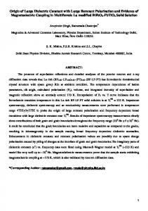
where 2𝛼 = 2𝛽𝑜 𝜅 is referred to as the absorption (or attenuation) coefficient and 1/2𝛼 is the mean free path length. Here, the medium’s opacity or optical depth (or thickness), 𝜏 = −𝑙𝑛{𝒯0 } = 2𝛼𝑙 for a homogeneous material, is dimensionless (i.e., not a physical length). A photon with energy ℎ𝑓, where ℎ is the Planck constant, on average is absorbed with 𝜏(𝑓) = 1. Here, 𝒯0 ≃ 37% (having a reflection-less insertion loss of -4.34 dB) and with no reflections then absorptance 𝒜0 ≃ 63% . When 𝜏(𝑓) < 1 a medium is considered here to be (semi)transparent and when 𝜏(𝑓) < 0.1 transparent (or optically thin, with a reflection-less insertion loss above -0.434 dB). Conversely, when 𝜏(𝑓) > 1 a medium is considered here to be (semi-)opaque and when 𝜏(𝑓) > 10 opaque (or optically thick, with a reflection-less insertion loss below -43.4 dB). This transmittance approximation inherently makes the unrealistic assumption that the sample under test has no reflections at its boundaries. Nevertheless, this over-simplified model provides useful variables for the more realistic models that follow. B. Power Propagation Model Approximate expressions for reflectance, transmittance and absorptance/emissivity were derived for a non-opaque sample having a physical temperature (i.e., above absolute zero) by McMahon [7]. The resulting model is given in terms of both zero-order reflectance and transmittance, while also considering multiple (i.e., higher order) reflections at its boundaries. Our heuristic engineering approach is much simpler and gives the same results. With reference to a non-opaque sample, illustrated in Fig. 1, the reflected power from the first-order reflectance ℛ1 = ℛ0 at the first boundary is 𝑃𝑟1 = ℛ0 𝑃𝑖 . A fraction 𝒯10 = (1 − ℛ0 ) of the incident power penetrates the first boundary. This proportion is reduced to 𝒯10 𝒯0 after propagating across the sample. A proportion 𝒯01 of the remaining power penetrates the second boundary. The resulting transmitted power from the first-order transmittance 𝒯1 = 𝒯10 𝒯0 𝒯01 at the second boundary is 𝑃𝑡1 = 𝒯1 𝑃𝑖 . The remaining reflected power at the second boundary has a fraction 𝒯10 𝒯0 ℛ0 of the incident power. Hence, the reflected power due to the second-order reflectance ℛ2 = 𝒯10 𝒯0 ℛ0 𝒯0 𝒯01 at the first boundary is 𝑃𝑟2 = ℛ2 𝑃𝑖 . Once again, a portion of power is reflected back into the sample, giving rise to an infinite number of Fabry-Perot reflections. The sum of these contributions is represented by the overall (or apparent [7]) reflectance,

Fig. 1. Heuristic engineering approach to the power propagation model: (top) illustrating individual contributions; (bottom) illustrating Fabry-Perot reflections.

where the overall (or apparent [7]) transmittance 𝒯 resulting from an infinite number of Fabry-Perot reflections is given as, 𝒯=

𝑃𝑡 𝑃𝑖

≈

∑∞ 𝑚=1 𝑃𝑟𝑚 𝑃𝑖

𝑝=∞

= (1 − ℛ0 )2 𝒯0 ∑𝑝=0 (ℛ0 𝒯0 )2𝑝

⇒

(1−ℛ0 )2 𝒯 1−(ℛ0 𝒯0 )2 0

(5)

The absorptance 𝒜 can also be equating to emissivity ℰ when derived from first principles by considering a slab in thermodynamic equilibrium [7]. More simply, however, it can be found by directly applying the principle of conservation of energy, such that, ℛ+𝒯+𝒜 =1

(6)

By inserting (4) & (5) into (6), absorptance is given by, 𝒜=

(1−ℛ0 )(1−𝒯0 ) 1−ℛ0 𝒯0

(7)

As a sanity check, absorptance can only be zero when the sample under test is either a perfect electrical conductor (PEC), such that all the incident radiation is reflected (i.e., ℛ = 1 and 𝒯 = 0 with ℛ0 = 1), or free space, such that all the incident radiation is transmitted (i.e., ℛ = 0 and 𝒯 = 1 with ℛ0 = 0 and 𝒯0 = 1), as illustrated in Fig. 2 [9].

Fig. 2. Interplay of ℛ , 𝒯 and 𝒜 = ℰ , as they vary in relation to one another for 1 mm thick slabs of various materials at 29, 60 and 600 THz [9].



4 C. Full-spectrum Power Response Modeling Example The highly cited work of Rubin [10] illustrates some of the challenges associated with accurately extracting effective complex dielectric properties using power response measurements. The dielectric slabs under investigation were various types of window glass; the same sample being both optically thick within the far infrared and optically thin within the near infrared and visual spectra. Since window glass was known, a priori, to be (semi)opaque below ca. 60 THz [10], it is reasonable to assume that there will be no significant transmittance and, therefore, no observable Fabry-Perot resonances. For this reason, only reflectance measurements were performed, from 6 to 100 THz, using a thermal infrared IBM Fourier-transform spectrometer (at near-normal incidence); extrapolation assumptions were also made below 6 THz [10]. This allowed Rubin to adopt the zero-order model for reflectance ℛ0 . The Kramers-Krönig or dispersion equation shows the dependent relationship between the real and imaginary parts of an analytic function, such as those associated with complex dielectric properties [11]. For example, the amplitude |𝜌| and phase angle ∠𝜌 for the overall electric-field wave reflection coefficient 𝜌 = |𝜌|𝑒 +𝑗∠𝜌 are related to one another through Kramers-Krönig integrals. Rubin uses this technique for extracting the phase spectra from reflectance ℛ ≅ ℛ0 = |𝜌0 |2 measurements as, ∠𝜌0 (𝜔) =

𝜔

+∞ 𝑙𝑛{ℛ0 (𝜔 ̅ )}

∫ 𝜋 0

̅ 2 −𝜔2 𝜔

∙ 𝑑𝜔 ̅

(8)

With both ℛ0 and ∠𝜌0 , the optical constants can be extracted, 𝑛̃ ≅ 𝑛 ≅ (1+ℛ

1−𝜌0 1+𝜌0

(1−ℛ0 ) 0 )−2√ℛ0 cos(∠𝜌0 )

2√ℛ0 sin(∠𝜌0 )

𝜅 ≅ (1+ℛ

0 )−2√ℛ0 cos(∠𝜌0 )

(9) (10) (11)

Using Kramers-Krönig integrals with the zero-order model, the effective complex dielectric properties for typical clear window glass were extracted between 1 and 60 THz [10] and shown in Fig. 3. The vibrational absorption resonance frequencies at approximately 14.3 and 31.5 THz were attributed to Si-O bending and stretching [10], clearly seen in Fig. 3. Since window glass was known, a priori, to be (semi)transparent above ca. 65 THz [10], it is reasonable to assume that there will be significant transmittance and, therefore, observable Fabry-Perot resonances. For this reason, the backside surface of the samples (i.e., at the second boundary) were roughened to ‘prevent’ Fabry-Perot resonances above 65 THz [10]. Between 65 and 967 THz, conventional reflection and transmission mode power measurements were undertaken at normal incidence. However, in this frequency range, Rubin adopts an empirical-fit dispersion equation for 𝑛 [12]. For 𝜅, once again, Rubin only adopts the zero-order model for reflectance ℛ0 . However, in addition, the power propagation

model for transmittance 𝒯, defined for an infinite number of Fabry-Perot reflections, was used. With both ℛ0 and 𝒯, (5) can be rearranged to extract 𝜅, 𝜅=−

𝜆𝑜 4𝜋𝑙

𝑙𝑛{𝒯0 }

(12)

where, 𝒯0 =

√(1−ℛ0 )4 +(2ℛ0 𝒯)2 −(1−ℛ0 )2 2ℛ02 𝒯

(13)

Fig. 3. Published complex refractive index (and associated effective complex relative permittivity) for typical clear window glass [10] (circular and triangular data points represent correct solutions extracted using our two and three equation methods, respectively, discussed in Sections VI and VII).

Using the empirical-fit dispersion equation for 𝑛, the zeroorder model for reflectance and the power propagation model for transmittance, the effective complex dielectric properties for typical clear window glass were extracted between 65 and 100 THz [10] and shown in Fig. 3. Clearly, the ultimate accuracy of the dataset in Fig. 3 is uncertain, due to: (i) experimental limitations in both of Rubin’s 1980’s measurement setups – Fourier-transform spectrometer within the thermal infrared (operating 6 and 100 THz) and conventional power measurements within the solar spectrum (operating between 65 and 967 THz) – which include ambient atmospheric conditions (e.g., absorber concentration levels, temperature and pressure [3]), systematic errors (e.g., mechanical and calibration accuracy) and random errors (surface roughness uniformity/repeatability, detector noise and any limits in mathematical precision); (ii) approximations used with the extreme extrapolations, due to the absence of measured spectral data from dc to infinity required by the zero-to-infinity bounds of the Kramers-Krönig integrals [11], although Riu and Lapaz [13] conclude that these relations are practical in almost every experimental situation [14]; and within the solar spectrum (iii) inherent errors in the use of the empirical equation for 𝑛; (iv) the specular reflections from the optically flat front-side surface gives a zero-order reflectivity ℛ0 , while diffuse reflections from the roughened backside surface (with unspecified surface roughness) gives an effective zero-order ⃛0 < ℛ0 – while the sample under test is still reflectivity ℛ ⃛0 needs to be reciprocal, it is no longer symmetrical and so ℛ characterized and taken into account; (v) adopting the zeroorder model, instead of the more accurate power propagation reflectance model, which now requires (4) to be modified for



5 ⃗ (and for completeness the the first boundary reflectance ℛ ⃖⃗), second boundary reflectance ℛ 2𝒯 2 0 1−ℛ0 ℛ0 𝒯02

⃗ ⇒ ℛ0 + (1−ℛ0 ) ℛ ⃛

⃛ 2 𝒯02

⃛0 and ℛ ⃖⃗ ⇒ ℛ ⃛0 + (1−ℛ0 ) ℛ ⃛

1−ℛ0 ℛ0 𝒯02

ℛ0 (14)

and (vi) adopting the power propagation transmittance model, which now requires (5) to be modified to, 𝒯⇒

⃛0 ) (1−ℛ0 )(1−ℛ 𝒯0 ⃛0 𝒯02 1−ℛ0 ℛ

(15)

For completeness, inserting (14) & (15) into (6), reveals the modified absorptance as, 𝒜⇒

⃛0 𝒯0 )(1−𝒯0 ) (1−ℛ0 )(1+ℛ ⃛0 𝒯02 1−ℛ0 ℛ

Consider the electric field 𝐸𝑖 incident at the first boundary of the sample. A portion of the incident wave energy is reflected back, giving the first-order electric field term 𝐸𝑟1 = 𝜌0 𝐸𝑖 . The portion penetrating the first boundary has an electric field 𝜏10 𝐸𝑖 , which then propagates across the sample. The electric field arriving at the second boundary is 𝜏10 𝑒 −𝛾𝑙 𝐸𝑖 . The associated energy is then split into two parts; one portion is reflected backwards and the rest penetrates the second boundary. The former contributes to the infinite number of internal Fabry-Perot reflections. With the latter, the electric field emerging from the sample is denoted by the first-order electric field term 𝐸𝑡1 = 𝜏10 𝑒 −𝛾𝑙 𝜏01 𝐸𝑖 , which contributes to the externally measured signal.

(16)

Clearly, when compared to using (12) & (13) directly, extracting optical constants with (14) & (15) is no longer straightforward. Nevertheless, while not definitive, Rubin’s combined dataset for typical clear window glass (given in Fig. 3) is arbitrarily adopted within this paper as a useful benchmark for performing mathematically traceable simulations; its optical constants have a conveniently wide range of values across our 1 to 100 THz spectral range of interest. IV. EXACT POWER RESPONSE MODELING A. Electric Field Propagation Model (EFPM) In Section III, it was shown how the dielectric sample under test can behave as a Fabry-Perot resonator. With terahertz timedomain spectroscopy, this resonator can be excited by a short pulse of THz radiation incident on the slab. The externally measured signals have temporal features that are dependent on the multiple internal reflections at its boundaries. Theses multiple reflections can be seen as a series of delayed echoes within the time domain. Consider the non-opaque sample illustrated in Fig. 4, after applying Fourier transforms to the THz TDS measurements. The intrinsic impedances of free space and non-magnetic materials are 𝜂0 and 𝜂 , respectively, where 𝜂 = 𝜂0 /𝑛̃ . At normal incidence, the complex Fresnel reflection coefficients for electric field waves travelling from left to right, at the respective first and second boundaries are, 𝜌0 = 𝜌1 =

𝜂−𝜂0 𝜂+𝜂0

𝜂0 −𝜂 𝜂0 +𝜂

=

=

1−𝑛̃

(17)

1+𝑛̃

𝑛̃−1 𝑛̃+1

= −𝜌0

(18)

Also, at normal incidence, the complex Fresnel transmission coefficients, for electric field waves travelling from left to right, at the respective first and second boundaries are, 2

𝜏10 = 1 + 𝜌0 =

1+𝑛̃

𝜏01 = 1 + 𝜌1 =

1+𝑛̃

2𝑛̃

(19) (20)

Fig. 4. Heuristic engineering approach to the field propagation model: (top) calibration; (middle) illustrating individual contributions; (bottom) illustrating Fabry-Perot reflections.

Two reference electric field measurements, identified by the ref subscript (seen at the top of Fig. 4), are needed to effectively calibrate the spectrometer. The first extracts the Fresnel reflection coefficient of a typically gold-coated mirror 𝜌𝑚 ≅ −1 (approximating 𝜌𝑚 = −1 from a PEC) at the location of the first boundary. The second determines the propagation through free space between the two boundaries (i.e., approximating the phasor 𝑒 −𝑗𝛽0𝑙 between the measurement reference planes), governed by the thickness 𝑙 of the sample under test, 𝐸𝑟𝑟𝑒𝑓 = 𝜌𝑚 𝐸𝑖 ≅ −𝐸𝑖

(21)

𝐸𝑡𝑟𝑒𝑓 ≅ 𝐸𝑖 𝑒 −𝑗𝛽0 𝑙

(22)

With THz TDS, in theory, coherent pulse echoes due to internal Fabry-Perot reflections can be separated out in time. Depending on the frequency dispersion encountered by the pulse, it will have a pulse width 𝑡𝑤 ≲ 2𝑛𝑙/𝑐, For example, in theory, 𝑡𝑤 ≲ 5 ps with a sample having an assumed index of refraction 𝑛 =1.5 and thickness 𝑙 = 500 µm. The non-resonant model can be obtained by applying a time window (also known as time gating with time-domain reflectometry (TDR) [15]) to capture just the first reflected and transmitted pulses to emerge from the samples [16] [17]. After applying Fourier transforms, the resulting complex first-order



6 reflection and transmission transfer functions (or coefficients) are, respectively, given by, 𝐻𝑅1 = 𝐻𝑇1 =

𝐸𝑡1 𝐸𝑡𝑟𝑒𝑓

≅

𝐸𝑟1 𝐸𝑟𝑟𝑒𝑓

≅ −𝜌0 =

𝜏10 𝑒 −𝛾𝑙 𝜏01 𝑒 −𝑗𝛽0 𝑙

=

𝑛̃−1

(23)

𝑛̃+1

4𝑛̃ (𝑛̃+1)2

𝑒 −𝑗𝛽0(𝑛̃−1)𝑙

(24)

It will now be shown that the optical constants can be extracted (in this case recovered) using transmission mode THz TDS using (24), where MEAS subscripts refer to measured variables, as follows, 𝑛 = 1+

1 ∠𝜏10 (𝑛̃)+∠𝜏01 (𝑛̃)−∠𝐻𝑇𝑀𝐸𝐴𝑆

𝛽𝑜 𝑙

𝜅=−

𝑙𝑛{|𝜏

|𝐻1 𝑇𝑀𝐸𝐴𝑆 |

̃ )||𝜏01 10 (𝑛

𝛽𝑜 𝑙

} (𝑛 ̃ )|

≅ 1−

1 ∠𝐻𝑇𝑀𝐸𝐴𝑆

𝛽𝑜 𝑙

(25)

2

1 1 (𝑓)|) − 𝑙𝑛(|𝐻𝑇𝑀𝐸𝐴𝑆 (𝑓)|)) 𝐸𝑟𝑟𝑜𝑟(𝑛̃, 𝑓) = (𝑙𝑛(|𝐻𝑇𝑆𝐼𝑀

|𝐻1 𝑇𝑀𝐸𝐴𝑆 |

≅−

𝑙𝑛{ 𝑇 (𝑛) } 𝐹 𝛽𝑜 𝑙

1 amplitude and phase information (where 𝐻𝑅𝑀𝐸𝐴𝑆 is the measured complex first-order reflection transfer function), which can be used to find the two unknown optical constants. With the former, more cumbersome reflection mode measurements, (23) can be solved directly to extract the exact optical constants as there is no 𝑒 −𝑗𝛽𝑜 𝑛𝑙 ambiguity to consider. However, in practice, phase information is not normally available in the reflection mode. With the latter, more simple transmission mode measurements, (24) cannot be solved directly due to the 𝑒 −𝑗𝛽𝑜 𝑛𝑙 ambiguity. Equation (24) can be solved by using numerical iterative methods, but only when given an initial guess that is very close to the final solution. An approximation method, without requiring an initial guess, was proposed by Duvillaret et al. [20]. They defined a smooth and monotonic error function as,

2

1 1 (𝑓) − ∠𝐻𝑇𝑀𝐸𝐴𝑆 (𝑓)) +(∠𝐻𝑇𝑆𝐼𝑀

(26)

1 where 𝐻𝑇𝑀𝐸𝐴𝑆 is the measured complex first-order 1 | = |𝐸𝑡1𝑀𝐸𝐴𝑆 |/ transmission transfer function (with |𝐻𝑇𝑀𝐸𝐴𝑆 1 |𝐸𝑡𝑟𝑒𝑓𝑀𝐸𝐴𝑆 | and ∠𝐻𝑇𝑀𝐸𝐴𝑆 = ∠𝐸𝑡1𝑀𝐸𝐴𝑆 − ∠𝐸𝑡𝑟𝑒𝑓𝑀𝐸𝐴𝑆 ) and the Fresnel reflection loss 𝑇𝐹 (𝑛) = 𝜏10 (𝑛)𝜏01 (𝑛) = 1 − ℛ0 (𝑛) [18]. The approximate expressions for the extracted optical constants, 𝑛 with (25) and 𝜅 with (26), assume that both complex Fresnel transmission coefficients ( 𝜏10 and 𝜏01 ) are approximated by replacing the complex refractive index, seen in (19) and (20), with only the index of refraction [19]. The reason for doing this is that the extraction of 𝑛 no longer needs the Fresnel transmission coefficients, while for 𝜅 the approximated coefficients can be calculated using the extracted approximation for 𝑛. To test these approximations, we swept both target variables over the ranges of 1 ≤ 𝑛 ≤ 5 and 0 ≤ 𝜅 ≤ 0.07, for arbitrary sample thickness of 500 µm and frequency of 1 THz. Here, the dielectric has a worst-case loss tangent of 𝑡𝑎𝑛 𝛿 = 0.141 and sample opacity of 𝜏(1 THz) = 1.5 . With (25), it was first necessary to replace the wrapped with the unwrapped phase angle ∠𝐻𝑇1 ,

∠𝑒 𝑗[∠𝜏10(𝑛̃)+∠𝜏01(𝑛̃)−𝛽0(𝑛−1)𝑙] wrapped ∠𝐻𝑇1 = { (27) ∠𝜏10 (𝑛̃) + ∠𝜏01 (𝑛̃) − 𝛽0 (𝑛 − 1)𝑙 unwrapped It was found that the error between the original swept and extracted approximate values for 𝑛 [19] was below 0.06% for our worst-case values at 𝑛̃ = 1.62 − 𝑗0.07 ; which is well within experimental error. With (26), the approximation [19] is also very good, reaching a peak error of 0.16% for our worstcase values at 𝑛̃ = 1 − 𝑗0.07 . However, with both approximations, the errors increase with opacity. Other methods for extracting the effective complex dielectric properties are reported in [16] using (23) & (24) and [20] using just (24), requiring the combination of both amplitude and phase information. In general, measurements can be taken from either the first-order reflection or transmission mode measurements. This is because, in principle, with THz TDS, the 1 1 independent measurements of 𝐻𝑅𝑀𝐸𝐴𝑆 and 𝐻𝑇𝑀𝐸𝐴𝑆 both give

(28)

1 where SIM subscripts refer to simulated variables and 𝐻𝑇𝑆𝐼𝑀 is the simulated complex first-order transmission transfer function. This error function is similar to a paraboloid and can be approximated by the general equation for a paraboloid. Hence, the problem is to find the minima of the paraboloid, either analytically or numerically. By including more Fabry-Perot reflections (i.e., by expanding the time window), the respective overall reflected and transmitted electric fields from the sample are,

𝐸𝑟 = 𝜌0 𝐸𝑖 − 𝜏10 𝜏01 𝜌0 𝑒 −2𝛾𝑙 𝐸𝑖 − 𝜏10 𝜏01 𝜌0 3 𝑒 −4𝛾𝑙 𝐸𝑖 − ⋯ = [𝜌0 −

(1−𝜌𝑜2 ) 𝜌0

−𝛾𝑙 2𝑝 ∑𝑀 ) ] 𝐸𝑖 𝑝=1(𝜌0 𝑒

(29)

𝐸𝑡 = 𝜏10 𝜏01 𝑒 −𝛾𝑙 𝐸𝑖 + 𝜏10 𝜏01 𝑒 −𝛾𝑙 (𝜌0 𝑒 −𝛾𝑙 )2 𝐸𝑖 + 𝜏10 𝜏01 𝑒 −𝛾𝑙 (𝜌0 𝑒 −𝛾𝑙 )4 𝐸𝑖 + ⋯ −𝛾𝑙 2𝑝 = (1 − 𝜌𝑜2 )𝑒 −𝛾𝑙 ∑𝑀 ) 𝐸𝑖 𝑝=0(𝜌0 𝑒

(30)

−𝛾𝑙 2𝑝 where the power series term ∑𝑀 ) is sometimes 𝑝=0(𝜌0 𝑒 referred to as the Fabry-Perot (FP) factor [21]. Hence, in terms of the complex refractive index, the corresponding transfer functions are,

𝐻𝑅𝐹𝑃 =

𝐸𝑟 𝐸𝑟𝑟𝑒𝑓

𝐻𝑇𝐹𝑃 =

≅ 𝐻𝑅1 + 𝐸𝑡 𝐸𝑡𝑟𝑒𝑓

4𝑛̃ 1−𝑛̃2

∑𝑀 𝑝=1 (

≅ ∑𝑀 𝑝=0 (

1−𝑛̃ 1+𝑛̃

1−𝑛̃

𝑒 −𝑗𝛽0𝑛̃𝑙 ) ̃

1+𝑛

𝑒 −𝑗𝛽0 𝑛̃𝑙 )

2𝑝

𝐻𝑇1

2𝑝

(31)

(32)

Note that the integer M represents the theoretical maximum number of Fabry-Perot round-trip reflections that can be captured by an expanded time window. Depending on the frequency dispersion encountered by the pulse, the period of the pulse train 𝑡𝑝 ≳ (1 + 2𝑀)𝑛𝑙/𝑐 ≳ (𝑀 + 0.5) 𝑡𝑤 . For example, a typical THz TDS system can generate femtosecond pulses with an 80 MHz repetition rate [22]; in theory, capturing M =



7 2,498 for a transparent sample having an assumed index of refraction 𝑛 =1.5 and thickness 𝑙 = 500 µm. With conventional frequency- and space-domain spectroscopy, 𝑀 → ∞ in (31) & (32), hence, the respective overall reflection and transmission transfer functions for the sample are, 𝐻𝑅𝐹𝑃 ⇒ [

1−𝑒 −2𝛾𝑙

1−(𝜌0 𝑒 −𝛾𝑙 )2

𝐻𝑇𝐹𝑃 ⇒

] 𝐻𝑅1

𝐻𝑇1

1−(𝜌0 𝑒 −𝛾𝑙 )2

(33) (34)

B. Voltage-wave Propagation Model (VWPM) A vector network analyzer (VNA), normally associated with general-purpose (i.e., not usually dedicated to material characterization) frequency-domain measurements up to ca. 1.5 THz measures scattering (or S)-parameters directly [23]. It has been previously shown for metals [24] and dielectrics [25] that the S-parameters for a 2-port network (e.g., overall input voltage-wave reflection coefficient 𝑆11 and overall forward voltage-wave transmission coefficient 𝑆21 ) are given by the transcendental equations, 𝑆11 = [ 𝑆21 =

1−𝑒 −2𝛾𝑙 1−(𝜌0 𝑒 −𝛾𝑙 )2

𝜏10 𝑒 −𝛾𝑙 𝜏01 1−(𝜌0 𝑒 −𝛾𝑙 )2

] 𝜌0 ≡ −𝐻𝑅𝐹𝑃

(35)

≡ 𝐻𝑇𝐹𝑃 𝑒 −𝑗𝛽0𝑙

(36)

Note that (35) and (36) have also been expressed in a similar form [26]. For the general spectroscopy scenario considered here, the S-parameter reference impedance is the intrinsic impedance of free space 𝜂0 . A much simpler and cheaper scalar network analyzer would measure |𝑆11 |2 and |𝑆21 |2 directly. From the equivalences given in (35) & (36), with conventional frequency-domain spectroscopy, the respective reflectance and transmittance for the sample are, |2

(37)

𝒯 = |𝐻𝑇𝐹𝑃 |2 ≡ |𝑆21 |2

(38)

ℛ = |𝐻𝑅𝐹𝑃

|2

≡ |𝑆11

Measurements from a network analyzer directly applies the principle of conservation of energy to give, 𝒜 = 1 − |𝑆11 |2 − |𝑆21 |2

(39)

Once again, absorptance can only be zero when the sample under test is either a PEC (i.e., ℛ = 1 and 𝒯 = 0 with 𝜌0 = 1) or free space (i.e., ℛ = 0 and 𝒯 = 1 with 𝜌0 = 0 and 𝑒 −𝛾𝑙 = 𝑒 −𝑗𝛽0𝑙 ). It is interesting to note that the same exact closed-form expressions for the S-parameters can also be obtained by applying Mason’s non-touching loop rule [27] to the signal flow graphs shown in Fig. 5. This was originally demonstrated by Nicolson and Ross in 1970 [28], using the signal flow graph shown in Fig. 5(a). However, this model is not intuitive nor unilateral (i.e., it inherently assumes symmetry in the sample). For this reason, we propose the complete model given in Fig. 5(b). Our bilateral signal flow graph has the advantage in that it

can be easily modified to be non-symmetrical and expanded to cater for a laminated material system, while still being intuitive (unlike the use of transmission matrix methods). For example, the sample under test may be a conductive thin-film (e.g., using reflection mode space-domain spectroscopy [29]) or 2D metamaterial (e.g., using transmission mode THz TDS [17]) that is deposited with a thickness 75%. Moreover, the zero-order and power propagation models fit the exact models, as seen by the very low calculated errors given in Fig. 10. There is a sharp spectral feature at 1 THz, which may be an artifact from the extrapolation assumptions below 6 THz [10]. From ca. 65 THz up to 100 THz, it is confirmed that typical clear window glass is (semi-)transparent with 𝒯 increasing from ~33% to an average of ~75% and 𝒜 falling from ~62% to an average of ~15%. As a result, significant spectral ripples (due to the constructive and destructive interference associated with Fabry-Perot resonances; characteristic maxima in the reflection spectrum coincide with minima in the transmission spectrum) can be seen with the exact models, as they take into account phase information However, without phase information, no spectral ripples are seen with the zero-order or power propagation models. The least accurate zero-order model gives inflated transmittance and deflated absorptance spectral results, showing errors of up to 10 %, in this example, when compared to those from the more accurate power propagation model.

Fig. 10. Errors in calculated normalized power spectra with zero-order (dotted) and power propagation (dashed) models, relative to the exact models.

VI. SINGLE SOLUTION AND THRESHOLD ANALYSIS Extracting the correct values for effective dielectric properties is problematic due to the ambiguity introduced by the 𝑒 −𝑗𝛽0 𝑛𝑙 phasor term, found with both reflection and transmission mode measurements, embedded within the transcendental equations (33) to (36), generating multiple mathematical solutions. A. Vector Measurements With numerical methods, effective complex dielectric properties can be extracted from the combination of amplitude and phase measurements from the overall reflection and/or transmission transfer functions using (33) & (34) or full 2-port S-parameters using (35) & (36) with EFPM and VWPM or (46) & (47) using TLM. In their highly cited paper [28], Nicolson and Ross report on a ‘synthetic’ frequency-domain technique. They essentially take the discrete Fourier-transform (DFT) of time-domain reflectometry measurements to give complex frequencydomain S-parameters between 0.4 and 9.6 GHz. Placed within an air-filled coaxial transmission line medium, the first boundary of the sample under test is located a distance 2L from

a signal sampling head; while the second boundary is located at a distance L from a transmission back short circuit. These delay line lengths (with L = 375 mm) are long enough so that the measured incident, reflected and doubly-transmitted transientvoltage waveforms do not overlap at the sampling head. The reflected and transmitted waveforms each have a time window of 2𝐿/𝑐 = 2.5 ns, over which it is assumed that there is no contamination by other reflections. For example, with √2 ≤ 𝑛 ≤ 2 , the corresponding maximum truncated number of round-trip reflections captured for 6.35 mm thick semitransparent samples is 30 ≲ 𝑀 ≲ 41; transparent materials will need long delay lines. With this approach, two reference TDR measurements are initially taken; the first with a reflection short circuit placed at the first boundary and the second uses the transmission back short circuit when the sample under test is removed to leave the air-filled coaxial transmission line. The sample under test is then inserted and two more measurements are made. From the DFTs of these four time-domain measurements, ratios are taken to give the frequency-domain 2

measurements of −𝑆11 and 𝑆21 𝑆12 𝑒 𝑗2𝛽0𝑙 = (𝑆21 𝑒 𝑗𝛽0𝑙 ) . The 2.5 ns time window was digitized with 256 discrete samples, giving a Nyquist (or folding) frequency of 51.2 GHz. However, while Nicolson and Ross note that the errors due to truncation and aliasing with their DFT approximation were insignificant [28], there are other sources of errors inherent with time-domain reflectometry; even more so with ‘synthetic-pulse’ TDR (whereby physical measurements are performed in the frequency domain and an inverse DFT is applied in order to perform time gating) [15]. Moreover, with higher dielectric constant samples, timing displacements cause significant errors as frequency increases. It is interesting to note here that the UK’s National Physical Laboratory (NPL) recently undertook an international inter-comparison of THz TDS, extracting the optical constants between dc and 3 THz for standard material slabs (including silicon, quartz, silica glass and HDPE) from 16 high-profile laboratories (including national measurement institutes, academia and THz system manufacturers) [34]. The conclusion drawn for THz TDS was that “these results clearly indicate that standardization of measurement techniques is necessary and urgent” [34]. For example, if the extracted optical constants vary with sample thickness then this indicates a systematic error in the basic metrology-extraction characterization process. This is evident in the work reported by Arscott et al., using transmission mode THz TDS [35]. With ultra-thick negative photoresist SU-8, the index of refraction and absorption coefficient were measured between 0.1 and 1.6 THz. At 1 THz, 𝑛̃(𝑙 = 520 𝜇𝑚) = 1.69 − 𝑗0.0483 and 𝑛̃(𝑙 = 620 𝜇𝑚) = 1.73 − 𝑗0.0494; representing a noticeable increase of 2.4% and 2.3% in the index of refraction and extinction coefficient, respectively, as the sample thickness increases by 19%. In addition, the spectral ripples they observe in the measured index of refraction and absorption coefficient, across the frequency range of interest, were attributed to “a slight lack of parallelism in the sample” [35]. From the resulting two ‘synthetic’ frequency-domain measurements, Nicolson and Ross then extract 𝜌0 and 𝑒 −𝛾𝑙 with (35) & (36), which inherently assumes 𝑀 → ∞, using a rather convoluted mathematical derivation. Finally, the



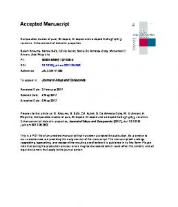
11 complex relative permeability and effective permittivity for 6.35 mm thick samples (including Teflon®, maple wood, nylon ′ and Plexiglas®, all having 2 ≤ 𝜀𝑟𝑒𝑓𝑓 ≤ 4 within their frequency range of interest) are extracted. However, their equation for 𝑛̃2 (i.e., their variable 𝑐2 with equation (9) in [28]) has an infinite number of roots when taking the natural logarithm of 𝑒 𝛾𝑙 ; there is an ambiguity because the phase of 𝑒 −𝛾𝑙 does not change when the sample thickness is increased by a multiple of wavelengths within the sample [36]. The ambiguity in phase must be resolved at each frequency by matching calculated and measured differential-phase group delay. Moreover, at frequencies corresponding to integer multiples of half a wavelength within the sample (with wavelength 𝜆 = 𝜆𝑜 /𝑛), reflectance is low (where 𝑆11 → 0 with a lossless material) and their 𝜌0 and 𝑒 −𝛾𝑙 become unstable [37] [38]. For this reason, sample thickness must be constrained to 𝑙 < 𝜆/2 (i.e., optical path length 𝑛𝑙 < 𝜆0 /2 ), increasing measurement uncertainty [37]. The US National Institute of Standards and Technology (NIST) solved this problem, to allow for any sample thickness, by applying numerical methods (Newton-Raphson iteration) with an initial guess for permittivity [37]. The real and imaginary parts of the effective complex relative permittivity for typical clear window glass have been extracted using the Nicolson and Ross method for various sample thicknesses ( 𝜆(100 THz)/2 , 3𝜆(100 THz)/4 , 𝜆(100 THz) , 5𝜆(100 THz)/4 and 3𝜆(100 THz)/2) and compared with the correct values taken from Fig. 3, with results shown in Fig. 11.

(a)

(b) Fig. 11. Extracted values of effective complex relative permittivity using the Nicolson and Ross method for typical clear window glass: (a) real part; and (b) imaginary part.

Over the frequency range of interest 𝑙𝑚𝑎𝑥 = 𝜆𝑚𝑖𝑛 /2 ⟶ 1 µm, in our case 𝜆𝑚𝑖𝑛 corresponds to a frequency of 100 THz and 𝑛(100 THz) = 1.5. It can be seen that when the sample thickness is only 1 μm (in practice it is very difficult to thin typical clear window glass to this thickness) then the Nicolson and Ross method generally recovers the correct values for 𝜀̃𝑟𝑒𝑓𝑓 from dc to 100 THz. However, an error can be seen between ca. 31 to 33 THz. Within this frequency interval, 𝜅 > 𝑛 and (51) ′ shows that 𝜀𝑟𝑒𝑓𝑓 < 0 . As a result, the final expression for permittivity (i.e., their equation (10) in [28]) can automatically choose the wrong root from the square root of a complex number, giving −𝜀̃𝑟𝑒𝑓𝑓 , as seen in Fig. 11. As thickness increases beyond 𝑙𝑚𝑎𝑥 , significant discrepancies can be seen between the results from Nicolson and Ross and the correct values. It is also interesting to note that ′ the periodic singularities in 𝜀𝑟𝑒𝑓𝑓 [37] [38], corresponding to integer multiples of half a wavelength within the sample, are not observed with our graphical approach (discussed later). Using a THz VNA, Hammler et al. recently reported a nondestructive testing methodology for simultaneously determining both the sample’s thickness 𝑙 and pure dielectric property of 𝜀𝑟′ [33]. A constrained nonlinear optimization process was employed to minimize the discrepancy between the simulated 𝑆21𝑆𝐼𝑀 (𝑓), using (36), and measured sample under test 𝑆21𝑀𝐸𝐴𝑆 (𝑓), according to the residual sum of squares, 𝑓

𝐸𝑟𝑟𝑜𝑟(𝑙, 𝜀𝑟′ ) = ∑𝑓21|𝑆21𝑆𝐼𝑀 (𝑓) − 𝑆21𝑀𝐸𝐴𝑆 (𝑓)|2

(56)

where 𝑓1 and 𝑓2 are the respective lower and upper frequency limits of the VNA measurements. Here, the physical thickness of the samples (measured with calipers) and a realistic prediction for 𝜀𝑟′ were used as an initial guess, although a multiple-start global search was performed to eliminate the risk of finding local minima. The fixed combination of (𝑙, 𝜀𝑟′ ) that minimizes (56) is assigned to the sample under test. It should be noted that (36) assumes a non-magnetic (𝜇̃𝑟 = 1) sample and that the optimization process makes unrealistic assumptions of ′′ the sample being both lossless ( 𝜀𝑟𝑒𝑓𝑓 = 0 ), to reduce ′ calculation complexity, and nondispersive ( 𝜀𝑟𝑒𝑓𝑓 ⇒ 𝜀𝑟′ is frequency independent) over the measurement frequency range [33]. Nevertheless, good fits between 𝑓1 = 0.75 and 𝑓2 = 1.1 THz were reported, with the coefficient of determination R2 ranging between 0.972 and 0.990 for different sample materials (including polystyrene, silicon and GaAs). Another numerical methodology for extracting the effective complex relative permittivity, again using transmission mode VNA measurements, was very recently developed by Chang et al. [39]. Here, assuming a non-magnetic sample and applying a Newton iterative algorithm with (47), in terms of 𝜀̃𝑟𝑒𝑓𝑓 (𝑓), the following error function is minimized at each frequency, 𝐸𝑟𝑟𝑜𝑟( 𝜀̃𝑟𝑒𝑓𝑓 (𝑓) ) = 𝑆21𝑆𝐼𝑀 (𝜀̃𝑟𝑒𝑓𝑓 (𝑓) ) − 𝑆21𝑀𝐸𝐴𝑆 (𝜀̃𝑟𝑒𝑓𝑓 (𝑓) ) (57) Again with an initial guess, 𝜀̃𝑟𝑒𝑓𝑓 (𝑓) is updated with a reasonable increment until the error function converges; in their case to a preset error tolerance of 10−7 . However, a wrong



12 initial guess for 𝜀̃𝑟𝑒𝑓𝑓 (𝑓) will result in non-convergence. In practice, with non-polar dielectrics, very low frequency values of 𝜀̃𝑟𝑒𝑓𝑓 (𝑓) can be used as the initial guess, since its value will not change much below the first vibrational absorption resonance frequency (normally found within the infrared); although this information must be known a priori. However, crystalline structures and molecular solids that exhibit interfacial and space charges result in very low frequency dispersion. Furthermore, with dipolar dielectrics, their relaxation frequencies are found in the (sub-)microwave and millimeter-wave spectrum, again excluding the use of very low frequency value guesses for 𝜀̃𝑟𝑒𝑓𝑓 (𝑓). B. Scalar Measurements Extracting optical constants from power measurements only, using (37) & (38), is still problematic, due to the ambiguity from the 𝑒 −𝑗𝛽0 𝑛𝑙 phasor term. One obvious exception is in the case of a medium having zero reflections/scattering. For example, when predicting atmospheric attenuation under pristine conditions (having 𝑛 ≅ 1) at upper microwave frequencies and shorter wavelengths [3]. Here, 𝒯 ⟹ 𝒯0 = 𝑒 −2𝛽𝑜 𝜅𝑙 and so the extinction coefficient can be extracted directly from line-of-sight transmittance measurements. If only the first reflected and transmitted pulses to emerge from the sample are captured, as obtained with THz TDS, the simulated first-order voltage-wave reflection and transmission coefficients can be written as, 1 𝑆11𝑆𝐼𝑀 ≡ −𝐻𝑅1

and

1 𝑆21𝑆𝐼𝑀 ≡ 𝐻𝑇1 𝑒 −𝑗𝛽0𝑙

(58)

The optical constants 𝑛 and 𝜅 can now be calculated by simultaneously solving the following pair of equations,

by the red and blue curves, respectively. The intersection of these two curves (indicated within the inset of Fig. 12) represents the theoretical simultaneous solution for 𝑛̃. Within conventional frequency- and space-domain spectroscopy, the respective overall simulated voltage-wave reflection and transmission coefficients (35) & (36) can be rewritten in terms of 𝑛̃ as, ̃ 𝑙) (1−𝑛̃2 )(1−𝑒 −2𝑗𝛽0 𝑛

𝑆11𝑆𝐼𝑀 = (𝑛̃+1)2 𝑆21𝑆𝐼𝑀 = (𝑛̃+1)2

̃𝑙 −(1−𝑛̃)2 𝑒 −2𝑗𝛽0 𝑛

̃𝑙 4𝑛̃ 𝑒 −𝑗𝛽0 𝑛 ̃𝑙 −(1−𝑛̃)2 𝑒 −2𝑗𝛽0 𝑛

(61) (62)

Fig. 12. Calculated individual solutions for arbitrarily chosen 500 μm thick typical clear window glass and frequency of 60 THz (opacity 𝜏(60 THz) = 3.8) from the first-order normalized power response.

Similar to the approach used previously, with (59) & (60), the optical constants 𝑛 and 𝜅 can be calculated by simultaneously solving the following pair of equations, |𝑆11𝑆𝐼𝑀 (𝑛̃)|2 − ℛ𝑀𝐸𝐴𝑆 = 0

(63) (64)

1 |𝑆11𝑆𝐼𝑀 (𝑛̃)|2 − ℛ1𝑀𝐸𝐴𝑆 = 0

(59)

|𝑆21𝑆𝐼𝑀 (𝑛̃)|2 − 𝒯𝑀𝐸𝐴𝑆 = 0

1 1 |𝑆21𝑆𝐼𝑀 (𝑛̃)|2 − 𝒯𝑀𝐸𝐴𝑆 =0

(60)

It will be found that plots for the individual solutions for 𝑛̃, with both (63) and (64), exhibit decaying ripples that result from the 𝑒 −𝑗𝛽0𝑛𝑙 phasor embedded within (61) and (62), respectively. However, ripples with overall transmittance are only observed with low opacity samples. The reason for the greater sensitivity to the 𝑒 −𝑗𝛽0𝑛𝑙 phasor with overall reflectance is that an pth-order transmittance requires one additional damped propagation of the electromagnetic wave (or guided-wave mode) through the lossy sample, when compared to the pth-order reflectance. At 5 THz, the index of refraction and extinction coefficient for typical clear window glass are 𝑛 = 2.199 and 𝜅 = 0.536, respectively [10], corresponding to an opaque medium at this frequency with 𝜏(5 THz) = 56.1. The corresponding emulated target values for ℛ𝑀𝐸𝐴𝑆 and 𝒯𝑀𝐸𝐴𝑆 for a 500 μm thick sample are approximately 16.39 % and 0 %, respectively (corresponding to a return loss of -7.9 dB and infinite insertion loss). With the same theoretical graphical method used previously, all individual solutions for 𝑛̃ are shown in Fig. 13, where individual solutions for (63) and (64) are represented by the red and blue curves, respectively. The red curve now exhibits decaying ripples that result from the 𝑒 −𝑗𝛽0𝑛𝑙 phasor embedded within (61). There is only one intersection from the plots for (63) and (64), which represents the single (exact)

1 where, ℛ1𝑀𝐸𝐴𝑆 and 𝒯𝑀𝐸𝐴𝑆 are the first-order normalized power measurements for reflectance and transmittance, respectively. With this simple scenario, the 𝑒 −𝑗𝛽0 𝑛𝑙 phasor term will not appear in the normalized power spectra using (23) & (24) and, therefore, there will be no ambiguities. It will be shown that by solving this pair of equations graphically then there will only be a single simultaneous solution for 𝑛̃ that is exact, unlike the approximation previously discussed for THz TDS. As a reference example, at 60 THz, the index of refraction and extinction coefficient for typical clear window glass are 𝑛 = 1.397 and 𝜅 = 0.003 [10], respectively, corresponding to a semi-opaque medium at this frequency (with 𝜏(60 THz) = 3.8). The corresponding emulated target values for ℛ1𝑀𝐸𝐴𝑆 and 1 𝒯𝑀𝐸𝐴𝑆 , calculated using (37) & (38) with (23) & (24), for a 500 μm thick sample are approximately 2.74% and 2.18% , respectively (corresponding to a return loss of -15.6 dB and insertion loss of -16.6 dB). With the graphical approach, we sweep both optical constants and separately plot the individual solutions for both (59) and (60), using the MATLAB ‘fimplicit function’ [40]. All individual solutions for 𝑛̃ are plotted in Fig. 12, where individual solutions for (59) and (60) are represented



13 simultaneous solution for 𝑛̃ , due to the high opacity of the sample elevating the blue curve above the background ripples of the red curve. Essentially, the single solution found from normalized power responses with frequency- and space-domain spectroscopy for an opaque medium is analogous to the single solution found from first-order normalized power responses with THz TDS. The reason is that with opaque materials, both the first-order reflectance dominates the overall reflectance (i.e., ℛ𝑀𝐸𝐴𝑆 ≅ ℛ1 ⟺ ℛ1𝑀𝐸𝐴𝑆 ) and the first-order transmittance dominates the 1 overall transmittance (i.e., 𝒯𝑀𝐸𝐴𝑆 ≅ 𝒯1 ⟺ 𝒯𝑀𝐸𝐴𝑆 ), as characterized by the non-resonant model.

Fig. 13. Calculated individual solutions for arbitrarily chosen 500 μm thick typical clear window glass and frequency of 5 THz (opacity 𝜏(5 THz) = 56.1) from the normalized power responses with frequency- and space-domain spectroscopy.

C. Scalar Measurements and 𝜅 − 𝑛 Threshold Analysis for the Thermal Infrared In this subsection, a unique empirical model is introduced using graphical techniques, which defines the threshold conditions that separates the region in 𝜅 − 𝑛 space that gives the single simultaneous solution for the complex refractive index from that which gives multiple mathematical simultaneous solutions. It has been shown that the intersection(s) of curves from (63) and (64) can be either single or multiple, depending on the opacity and its contribution from the extinction coefficient 𝜅. It is useful, therefore, to know the threshold for 𝜅 𝑇 , for a given 𝑛. As a result, there will only be one intersection of the curves from (63) and (64) for 𝜅 ≥ 𝜅 𝑇 . In this single solution space, it will be shown that our graphical method for extracting the complex refractive index works only for (semi-)opaque samples (i.e., 𝜏(𝑓) > 1 and so, for a fixed frequency, relatively thin samples for when 𝜅 is high or relatively thick samples for when 𝜅 is low). The threshold 𝜅 𝑇 for a dielectric slab with arbitrary thickness of 500 μm and frequency of 5 THz are shown in Fig. 15, with 𝑛 swept over the range associated with most normal dielectric materials of 1 ≤ 𝑛 ≤ 5. The blue circular data points indicate discrete samples [𝑛, 𝜅 𝑇 ] obtained by increasing 𝜅(𝑛) from zero to the threshold at which only one simultaneous solution exists for 𝑛̃; the black curve represents the corresponding empiricalfit threshold curve.

At 60 THz, however, typical clear window glass is only semiopaque with 𝜏(60 THz) = 3.8. The corresponding emulated target values for ℛ𝑀𝐸𝐴𝑆 and 𝒯𝑀𝐸𝐴𝑆 are approximately 2.84 % and 2.18 %, respectively (corresponding to a return loss of 15.5 dB and insertion loss of -16.6 dB). All individual solutions for 𝑛̃ are shown in Fig. 14. It can be seen that there are now 9 possible simultaneous solutions for 𝑛̃ within the limits of 1.39 < 𝑛 < 1.42. Without additional information, the correct simultaneous solution cannot be determined. Fig. 15. Discrete sampling data points for arbitrarily chosen 500 μm thick dielectric slab and frequency of 5 THz (giving 𝑁 ≅ 8.34), and the corresponding empirical-fit threshold curve.

As seen in Fig. 15, the empirical-fit equation for 𝜅 𝑇 (𝑛, 𝑁) |𝑆𝑖𝑛𝑢𝑠𝑜𝑖𝑑| consists of two terms; a rectified sinusoidal term 𝜅 𝑇 (its origin being the Fourier-transform of a unity height ‘top-hat’ function 𝑓(𝑛̅) having a width from -n to +n, giving a generic 𝐹(𝑛, 𝑁) = ℱ{𝑓(𝑛̅)} = 2𝑛{𝑠𝑖𝑛𝑐(2𝜋𝑛𝑁)} function with its first zero crossing at 𝑁 = 1/2𝑛 ) and an underlying trend term 𝜅 𝑇𝑇𝑟𝑒𝑛𝑑 , |𝑆𝑖𝑛𝑢𝑠𝑜𝑖𝑑|

Fig. 14. Calculated individual solutions for arbitrarily chosen 500 μm thick typical clear window glass and frequency of 60 THz (opacity 𝜏(60 THz) = 3.8) from the normalized power responses with frequency- and space-domain spectroscopy.

𝜅𝑇 = 𝜅𝑇 |𝑆𝑖𝑛𝑢𝑠𝑜𝑖𝑑| 𝜅𝑇

+ 𝜅 𝑇𝑇𝑟𝑒𝑛𝑑

(65)

𝜋 sin (2𝜋𝑁𝑛 − ) 1 1 4 }| = |( − ) ∙ 2𝑛 { 2 3𝜋 2𝜋𝑁𝑛 𝜋

= 𝐴0 |sin (2𝜋𝑁𝑛 − )| 4


(66)


14 𝜅 𝑇𝑇𝑟𝑒𝑛𝑑 = (1 − 𝑒 −𝐴1 (𝑛−1) ) ∙ (𝐴2 + 𝐴3 𝑛 − 𝐴4 𝑛2 )

(67)

where 𝐴0 (𝑁) = (1 − 2/3𝜋)/2𝜋𝑁 is the amplitude of the sinusoidal term and 𝑁 = 𝑙/𝜆0 > 1 is the dimensionless spatial frequency of the sinusoidal term (contained within the phasor term 𝑒 −𝑗𝛽0 𝑛𝑙 = 𝑒 −𝑗2𝜋𝑁𝑛 ), which quantifies the number of free space wavelengths between the measurement reference planes when the sample under test is removed. This is in contrast to the Nicolson and Ross method that requires 𝑁 ≤ 1/2𝑛. In addition, 𝐴1 , 𝐴2 , 𝐴3 and 𝐴4 are the variables associated with the trend term, all having the generic power law form 𝑎 ∙ 𝑁 𝑏 . Figure 16 shows the empirical-fit curves for 𝜅 𝑇𝑇𝑟𝑒𝑛𝑑 against 𝑛 based on the discrete sampling data points for an arbitrarily chosen 500 μm thick dielectric slab sample at various excitation frequencies between 5 and 200 THz; resulting in a good fit having 𝑅2 > 0.99 at each frequency. 𝐴1 (𝑁) = 0.1898 ∙ 𝑁 0.4207

(68)

𝐴2 (𝑁) = 0.0538 ∙ 𝑁 −0.7110

(69)

𝐴3 (𝑁) = 0.08527 ∙ 𝑁 −0.8608

(70)

𝐴4 (𝑁) = 0.005506 ∙ 𝑁 −0.7487

(71)

(b)

(c)

Fig. 16. Discrete sampling data points [𝑛, 𝜅𝑇𝑟𝑒𝑛𝑑 ] for an arbitrarily chosen 500 T μm thick dielectric slab at various excitation frequencies and the empirical-fit underlying trend curves.

(d) Fig. 17. Discrete sampling data points for variables against spatial frequency N and corresponding best-fit curves: (a) 𝐴1 with (68), (b) 𝐴2 with (69), (c) 𝐴3 with (70) and (d) 𝐴4 with (71).

The discrete sampling data points and the associated best-fit curves for 𝐴1 , 𝐴2, 𝐴3 and 𝐴4 against N are shown in Fig. 17; a good fit is obtained with a worst-case 𝑅2 ≥ 0.9957. It should be noted that our empirical model, with (65) to (71), is only valid for 1 ≲ 𝑛 ≲ 5 (fitting best with 𝑛 ≳ 1.30) and 8.33 < 𝑁 < 333.33 ; a more complicated expression for 𝜅 𝑇𝑇𝑟𝑒𝑛𝑑 is needed beyond these ranges.

The relationship between threshold 𝜅 𝑇 , 𝑛 and spatial frequency N is shown in Fig. 18. It can be seen that, for a fixed spatial frequency, the threshold 𝜅 𝑇 remains periodic along 𝑛, with the amplitude of the sinusoid 𝐴0 ∝ 1/𝑁. Moreover, for a fixed excitation frequency, thicker samples have a greater(smaller) single(multiple) solution space, when compared to thinner samples, because of the lower values for 𝜅𝑇 .

(a)

Fig. 18. Predicted 3D plot of threshold 𝜅𝑇 against 𝑛 and N.



15

The circular data points in Fig. 3 represent single (exact) solutions extracted (in this case recovered) for the complex refractive index and effective complex relative permittivity using our graphical technique. D. Scalar Measurements and Opacity Threshold Analysis It has been found that there is a minimum threshold value for opacity 𝜏 𝑇 that gives the single (exact) simultaneous solution for 𝑛̃ and this is a function of sample thickness. For example, with our arbitrarily chosen case of 𝑙 = 500 μm, 𝜏 𝑇 (𝑙 = 500 μm ) ≈ 7.2, which corresponds to a single simultaneous solution for all measurements from 2 to 42 THz (here, 𝜏(𝑓) ≳ 7.2 ). Similarly, with 𝜏 𝑇 (𝑙 = 36 mm ) ≃ 10.9 , a single simultaneous solution is obtained for all measurements from 1 to 100 THz (here, 𝜏(𝑓) ≳ 10.9). Inherently, it is not possible to find a simple scaling law for 𝜏 𝑇 (𝑙). For example, for a fixed sample thickness, if opacity falls below the threshold by a generic factor 𝑥 then the path length cannot be simply increased by 1/𝑥 to maintain the threshold opacity. The reason is that, by definition, opacity is derived from the zero-order approximation for transmittance 𝒯0 , which assumes no reflections at its boundaries. Therefore, as opacity falls below the threshold, higher order transmittance terms now contribute more to the overall transmittance and so the length generally needs to be increased by more than a factor of 1/𝑥; the extra path loss effectively compensates for the higher order contributions to the transmitted power through the sample.

Fig. 19. Heuristic engineering approach to the field propagation model with an ideal PEC mirror at the second boundary: (top) illustrating individual contributions; (bottom) illustrating Fabry-Perot reflections.

This can be verified by applying Mason’s non-touching loop rule to the corresponding signal flow graphs shown in Fig. 20. Equation (74) can be re-written in terms of 𝑛̃ as, ̃𝑙 (1−𝑛̃)−(1+𝑛̃)𝑒 −2𝑗𝛽0 𝑛

PEC 𝑆11𝑆𝐼𝑀 = (1+𝑛̃)−(1−𝑛̃)𝑒 −2𝑗𝛽0𝑛̃𝑙

(75)

VII. CORRECT SOLUTION FROM MULTIPLE SOLUTIONS SPACE It had been previously shown that, with our graphical method, multiple mathematical simultaneous solutions for the complex refractive index can be obtained from scalar measurements with frequency- and space-domain spectroscopy. In this section, with ideal metrology, the same theoretical graphical technique will be used to extract the correct values of optical constants, by introducing a simple additional measurement step. Consider a non-opaque sample under test with an ideal PEC back short circuit/mirror (or metallic coating on the backside surface) at the second boundary, as illustrated in Fig. 19. The Fresnel reflection coefficient at the second boundary becomes 𝑃𝐸𝐶 𝜌m = −1. When considering an infinite number of Fabry-Perot reflections, the respective overall reflected electric field and corresponding reflection transfer function for the sample are, 𝐸𝑟PEC = 𝜌0 𝐸𝑖 − 𝜏10 𝜏01 𝑒 −2𝛾𝑙 𝐸𝑖 − 𝜏10 𝜏01 𝜌0 𝑒 −4𝛾𝑙 𝐸𝑖 − ⋯ = [𝜌0 −

(1−𝜌𝑜2 ) 𝜌0

−2𝛾𝑙 𝑝 ∑∞ ) ] 𝐸𝑖 𝑝=1(𝜌0 𝑒

PEC 𝐻𝑅𝐹𝑃 ⇒ 𝐻𝑅1 +

(1−𝜌𝑜2 )𝑒 −2𝛾𝑙 1−𝜌0 𝑒 −2𝛾𝑙

Hence, the overall simulated PEC coefficient 𝑆11𝑆𝐼𝑀 is given as, PEC 𝑆11𝑆𝐼𝑀

=

𝑏1 𝑃𝐸𝐶 𝑎1

|

=

voltage-wave

𝜌0 −𝑒 −2𝛾𝑙 1−𝜌0 𝑒 −2𝛾𝑙

(72) (73) reflection

(a)

(b) Fig. 20. Signal flow graphs: (a) unique equivalence of the second boundary after applying a PEC mirror; (b) additional spectroscopy measurements with an ideal PEC mirror at the second boundary.

Equivalently, from transmission line theory with a short circuit termination at the output port, the input wave impedance is given by, PEC 𝜂𝐼𝑁 = 𝜂 tanh(𝑗𝛽0 𝑛̃𝑙) PEC 𝑆11𝑆𝐼𝑀 =

≡

PEC −𝐻𝑅𝐹𝑃

PEC 𝜂𝐼𝑁 −𝜂0 PEC +𝜂 𝜂𝐼𝑁 0

=

tanh(𝑗𝛽0 𝑛̃𝑙)−𝑛̃ tanh(𝑗𝛽0 𝑛̃𝑙)+𝑛̃

(74)


(76) (77)


16 In addition to (63) & (64), the optical constants 𝑛 and 𝜅 can now be calculated by simultaneously solving the following equation, 2

PEC PEC (𝑛̃)| − ℛ𝑀𝐸𝐴𝑆 |𝑆11𝑆𝐼𝑀 =0

(78)

analytically by exploiting a unique equivalence shown in Fig. 20(a). With the signal flow graph in Fig. 5(b), by inserting a voltage-wave reflection coefficient branch of -1 (i.e., representing a PEC mirror) between 𝑏2 and 𝑎2 , the result will be identical to that in Fig. 20(b).

All individual solutions for 𝑛̃, from (63), (64) & (78), for our 500 μm thick typical clear window glass at 60 THz, are shown in Fig. 21. The black curve represents solutions from (78), exhibiting decaying ripples that result from the 𝑒 −𝑗𝛽0𝑛𝑙 phasor term embedded within (75). It can be seen that any two of the three curves give multiple intersections. However, with ideal metrology, there is only one intersection for all the three curves, corresponding to the correct simultaneous solution (indicated within the inset of Fig. 21).

Fig. 22. Calculated individual solutions for arbitrarily chosen 500 μm thick typical clear window glass and frequency of 70 THz (opacity 𝜏(70 THz) = 0.3) from the normalized power responses with frequency- and space-domain spectroscopy, now including the reflectance with an ideal PEC mirror at the second boundary.

VIII. SINGLE SOLUTION SEARCH MINIMIZATION

Fig. 21. Calculated individual solutions for arbitrarily chosen 500 μm thick typical clear window glass and frequency of 60 THz (opacity 𝜏(60 THz) = 3.8) from the normalized power responses with frequency- and space-domain spectroscopy, now including the reflectance with an ideal PEC mirror at the second boundary.

Figure 22 shows all individual solutions for 𝑛̃ at 70 THz, where typical clear window glass is now semi-transparent with 𝜏(70 THz) = 0.3. The blue curve, now exhibiting ripples that result from the 𝑒 −𝑗𝛽0𝑛𝑙 phasor embedded within (62), moves down and creates a greater number of intersections. However, there will still always be only one correct solution simultaneously satisfying (63), (64) and (78); in this case at 𝑛 = 1.455 and 𝜅 = 0.00018. The triangular data points in Fig. 3 represent single (correct) solutions extracted (in this case recovered) for the complex refractive index and effective complex relative permittivity using our graphical technique, by introducing our third power response measurement for reflectance with a PEC at the second boundary. It has been shown that a scalar network analyzer requires three physical measurements to be performed to extract the exact complex dielectric properties. However, it is important to note that, a third measurement is not physically necessary if a VNA is employed, as it provides both amplitude and phase information with both reflection and transmission mode measurements. This is because, by mathematically short circuiting the output port of the two-port network, defined using the S-parameters from the original pair of reflection and transmission mode VNA measurements, the simulated PEC ‘measurement’ of ℛ𝑀𝐸𝐴𝑆 from the resulting one-port network can be conveniently emulated. This can be easily verified

Our graphical technique requires all the individual solutions to be determined before either visual inspection or applying numerical methods to find the single (correct) solution. As seen in Fig. 22, for transparent materials, there are many candidate simultaneous solutions from any two of the three equations with (63), (64) & (78). Minimizing the single solution search with an automated method of constraining 𝑛 will speed-up the extraction process. This can be done, in principle, with a general purpose VNA, having the ‘synthetic-pulse’ TDR option [15]. With band-pass(low-pass) frequency-domain operation, having an ideal ‘boxcar’(‘top-hat’ or ‘brick-wall’) filtering function with -3 dB bandwidth 𝐵𝑊 , the corresponding fullwidth at half-maximum (FWHM) values of the ‘syntheticpulse’ is 𝑡𝐹𝑊𝐻𝑀 = 1.2(0.6)/𝐵𝑊 [15]. With equal amplitude and time-unlimited 𝑠𝑖𝑛𝑐(𝑥) impulses, the theoretical timedomain response resolution is equal to the FWHM [15]. Assuming the sample under test is non-dispersive within the calibrated bandwidth of the frequency-domain measurements, with TDR, the time between the first and second reflected impulses 𝑡𝑟12 (corresponding to the first- and second-order reflections) gives the index of refraction from, 𝑡𝑟12 = 2𝑛𝑙/𝑐

(79)

The bounds for 𝑡𝑟12 are set by the response resolution between the second reflected impulse and both the first reflected impulse and the time aliasing interval of the first reflected impulse 𝑡𝐴 = 1/𝛿𝑓, where 𝛿𝑓 is the spectral frequency resolution, 𝑡𝐹𝑊𝐻𝑀 ≲ 𝑡𝑟12 ≲ (𝑡𝐴 − 𝑡𝐹𝑊𝐻𝑀 )

(80)

The time-domain response resolution limits the range of index of refraction to,



17 𝑐 1.2(0.6) 2𝑙

𝐵𝑊

≲𝑛≲

𝑐

(

1

2𝑙 𝛿𝑓

−

1.2(0.6) 𝐵𝑊

)

(81)

For example, with a VNA operating at W-band (75 to 110 GHz) and with 401 discrete frequency points, 𝐵𝑊 = 35 GHz and 𝛿𝑓 = 𝐵𝑊/(401 − 1) = 87.5 MHz. Therefore, with a 500 µm thick sample, 10.3 ≲ 𝑛 ≲ 3418 and this is well beyond our normal range, requiring either a thicker sample or an increase in measurement bandwidth. Our non-dispersion assumption is unrealistic in practice, but the extracted value for 𝑛 can be used as a useful approximation for narrowing down the search window with our graphical technique. IX. CONCLUSION Where suitable, THz TDS is the spectroscopists method of choice, not least because coherent pump-probe detection offers extremely high signal-to-noise ratio (S/N) [18], with excellent dynamic range [1], and the subsequent simplicity in extracting the complex dielectric properties from a sample under test. Unfortunately, (sub-)picosecond pulsed-laser based systems may be considered as a very expensive option, especially for just the occasional characterization of material samples. Moreover, the frequency resolution of THz TDS systems may be limited to the gigahertz range. A lower cost solution for the spectroscopist is to use either a dedicated frequency-domain CW-THz or low S/N space-domain FTIR spectrometer. For the non-spectroscopists, the use of existing general purpose frequency-domain vector network analysers would be the preferred option for material characterization, not least because of their extremely high S/N and sub-megahertz frequency resolution. However, as with CW-THz and FTIR spectroscopy, until now, there has been insufficient information from conventional reflection-transmission mode measurements for extracting complex dielectric properties with (semi)transparent samples. In this paper, we have undertaken a comprehensive (but not exhaustive) analytical review of reflection-transmission mode spectroscopy. Here, we use a consolidated framework of mathematical derivations for explaining the limitations of previously reported methods for extracting effective complex dielectric properties; such traceability being rarely considered. It should be noted that we deliberately chose not to include experimental validation for our work, in order to avoid introducing unnecessary systematic and random errors that are inherent with practical metrology. Instead, to provide full mathematical traceability, we adopt an arbitrarily chosen dataset, from 1 to 100 THz, to act as the reference for the effective complex dielectric properties of a sample under test. Normalized power spectra were simulated with the zero-order model, power propagation model and exact power response models; the results were then compared and contrasted. As expected, it was found that EFPM, VWPM, TLM and TE-TLM give the same numerical results and, thus, are considered as exact models. Significant discrepancies can be seen from the zero-order and power propagation models, due to the lack of phase information, and also the lack of Fabry-Perot reflections with the zero-order model. For extracting the effective complex dielectric properties, we present a detailed analysis of reported techniques that employ

either scalar or vector reflection-transmission mode measurements. It is found, in general, that only approximate values can be extracted with the use of numerical methods; requiring an initial guess and iterative solutions. Two exceptions (Smith et al. and also Nicolson and Ross) can extract the exact solution, but at the expense of either introducing multiple sample thicknesses or severely limiting the maximum thickness of the sample. Without any initial guesses, we report on a graphical technique that requires only one sample, of arbitrary thickness, to extract the exact optical constants. For an opaque medium, a pair of reflection-transmission mode measurements may be required; using either time-, frequency- or space-domain spectroscopy, without needing any phase information. A unique model is introduced using our graphical techniques, which defines the threshold conditions that separates the region in 𝜅 − 𝑛 space that gives the single simultaneous solution for the complex refractive index from that which gives multiple mathematical simultaneous solutions. Finally, with non-opaque media, in addition to the normal pair of reflection-transmission mode measurements, an extra reflection measurement is required employing a back short circuit or mirror. This is needed to resolve the 𝑒 −𝑗𝛽0 𝑛𝑙 phasor term ambiguity within the multiple solution space, giving the single (correct) solution. With three physical measurements even a scalar measurement system (e.g., low cost scalar network analyzer or FTIR spectrometer) can be used to extract the exact values. With a vector measurement system, the third measurement can be emulated by mathematically short circuiting the output port of the two-port network, defined by the S-parameters from the original pair of reflectiontransmission mode measurements. Finally, with our graphical technique requiring all the individual solutions to be determined, visual inspection for the simultaneous solution can be replaced by numerical methods for automated and/or real-time material characterization used in non-destructive testing.



18 APPENDIX In this errata appendix, typographical errors discovered in our cited references (found during the course of our derivations) are shown and corrected in Table 2. Note that the designated variables in Table 2 correspond to those from the original references. TABLE 2 SUMMARY OF TYPOGRAPHICAL ERRORS IN CITED REFERENCES

ACKNOWLEDGMENTS This work was supported in part by Imperial College MRC Confidence in Concept (ICiC) fund and NIHR Imperial BRC funding 2015/2016 and the UK’s Engineering and Physical Sciences Research Council (EPSRC) under Platform Grant EP/E063500/1. The authors would also like to thank Munir M. Ahmad, William J. Otter and Hang Ren (at Imperial College London) and Mira Naftaly (at the UK’s National Physical Laboratory) for their helpful discussions. REFERENCES [1] A. I. McIntosh, B. Yang, S. M. Goldup, M. Watkinson, and R. S. Donnan, “Terahertz spectroscopy: a powerful new tool for the chemical sciences?,” Chem. Soc. Rev., vol. 41, no. 6, pp. 2071-2082, Jan. 2012. [2] A. Mehta, Introduction to the Electromagnetic Spectrum and Spectroscopy (Analytical Chemistry), Pharmaxchange, Aug. 2011. [Online]. Available: http://pharmaxchange.info/press/2011/08/introduction-totheelectromagnetic-spectrum-and-spectroscopy/. [3] J. Sun, F. Hu, and S. Lucyszyn, “Predicting atmospheric attenuation under pristine conditions between 0.1 and 100 THz,” IEEE Access, vol. 4, pp. 93779399, Nov. 2016. [4] Terahertz Database. [Online]. Available: http://www.thzdb.org/. [5] B. T. W. Gillatt, M. D’Auria, W. J. Otter, N. M. Ridler, and S. Lucyszyn, “3-D printed variable phase shifter”, IEEE Micro. and Wireless Comp. Lett., vol. 26, no.10, pp. 822-824, Oct. 2016.

[6] J. Sun, F. Hu, Z. Wang, and S. Lucyszyn, “Banknote characterization using a thermal infrared ‘THz Torch’ spectrometer,” Asia-Pacific Microwave Conference (APMC2015), Nanjing, China, Dec. 2015. [7] H. O. McMahon, “Thermal radiation from partially transparent reflecting bodies,” J. Opt. Soc. Am., vol. 40, no. 6, pp. 376-380, June 1950. [8] B. L. Sopori, W. Chen, S. Abedrabbo, and N. M. Ravindra, “Modeling emissivity of rough and textured silicon wafers,” J. Elec. Mat., vol. 27, no. 12, Aug. 1998. [9] A. C. Jones, B. T. O’Callahan, H. U. Yang, and M. B. Raschke, “The thermal near-field: coherence, spectroscopy, heat-transfer, and optical forces,” Prog. Surf. Sci., vol. 88, no. 4, pp. 349-392, Dec. 2013. [10] M. Rubin, “Optical properties of soda lime silica glasses,” Sol. Energ. Mater., vol. 12, no. 4, pp. 275-288, Sep.-Oct. 1985. [11] S. Lucyszyn, “Investigation of anomalous room temperature conduction losses in normal metals at terahertz frequencies,” IEE Proc. Microw., Anten. Prop., vol. 151, no. 4, pp. 321-329, Aug. 2004. [12] M. Herzberger, “The dispersion of optical glass,” J. Opt. Soc. Am., vol. 32, no. 2, pp. 70-77, Feb. 1942. [13] P. J. Riu and C. Lapaz, “Practical limits of the Kramers-Kronig relationships applied to experimental bioimpedance data,” Ann. N.Y. Acad. Sci, vol. 873, pp. 374-380, Apr. 1999. [14] R. Kitamura, L. Pilon, and M. Jonasz, “Optical constants of silica glass from extreme ultraviolet to far infrared at near room temperature,” Appl. Opt., vol. 46, no. 33, pp. 8118-8122, Nov. 2007. [15] S. Lucyszyn, “RFIC and MMIC measurement techniques,” in Microwave Measurements, ch. 11, R. Collier and D. Skinner, 3rd Edition, London, IET, Oct. 2007, pp. 217-262. [16] H. Němec, F. Kadlec, P. Kužel, L. Duvillaret, and J.-L. Coutaz, “Independent determination of the complex refractive index and wave impedance by time-domain terahertz spectroscopy,” Opt. Commun., vol. 260, no. 1, pp. 175-183, Apr. 2006. [17] P. Kužel and H. Němec, “Metamaterials,” in Terahertz spectroscopy and imaging, ch. 22, K-E. Peiponen, J. A. Zeitler, and M. Kuwata-Gonokami, Heidelberg, Berlin, Springer, 2013, pp. 569-610. [18] M. Naftaly and R. E. Miles, “Terahertz time-domain spectroscopy for material characterization,” IEEE Proc., vol. 95, no. 8, pp.1658-1665, Aug. 2007. [19] W. Withayachumnankul and M. Naftaly, “Fundamentals of measurement in terahertz time-domain spectroscopy,” J. Infrared Milli. Terahz. Waves, vol. 35, no. 8, pp. 610-637, Aug. 2014. [20] L. Duvillaret, F. Garet, and J-L. Coutaz, “A reliable method for extraction of material parameters in terahertz time-domain spectroscopy,” IEEE J. Sel. Topics Quantum Electron, vol. 2, no. 3, pp. 739-746, Sep. 1996. [21] S. P. Mickan and X.-C. Zhang, “T-ray sensing and imaging,” in Terahertz sensing technology, Volume 1: Electronic devices and advanced systems technology, vol. 13, no. 2, D. L. Woolard, W. R. Loerop, and M. S. Shur, Singapore, World Scientific Publishing Co. Pte. Ltd., 2003, pp. 601-676. [22] I. Pupeza, R. Wilk, and M. Koch, “Highly accurate optical material parameter determination with THz time-domain spectroscopy,” Opt. Express, vol. 15, no. 7, pp. 4335-4350, Mar. 2007. [23] T. W. Crowe, J. L. Hesler, E. Bryerton, and S. A. Retzloff, “Terahertz sources and receivers for science applications and test & measurement systems,” IEEE Compound Semiconductor Integrated Circuit Symposium, Austin, USA, Oct. 2016. [24] S. Lucyszyn and Y. Zhou, “Characterising room temperature THz metal shielding using the engineering approach,” PIER, vol. 103, pp. 17-31, 2010. [25] F. Hu and S. Lucyszyn, “Modelling miniature incandescent light bulbs for thermal infrared ‘THz Torch’ applications,” J. Infrared Millim Terahertz Waves, vol. 36, no. 4, pp. 350-367, Apr. 2015. [26] L. M. Zurk and S. Schecklman, “Terahertz Scattering,” in Terahertz spectroscopy and imaging, ch. 5, K-E. Peiponen, J. A. Zeitler, and M. KuwataGonokami, Heidelberg, Berlin, Springer, 2013, pp. 569-610. [27] S. J. Mason, “Feedback theory-further properties of signal flow graphs,” Proc. IRE, vol. 44, no. 7, pp. 920-926, Jul. 1956. [28] A. M. Nicolson and G. F. Ross, “Measurement of the intrinsic properties of materials by time-domain techniques,” IEEE Trans. Instrum. Meas., vol. IM19, no. 4, pp. 377-382, Nov. 1970. [29] U. Nowak, J. Saalmüller, W. Richter, M. Heyen, and H. Janz, “Characterisation of the interface between GaAs:Cr substrates and n-type epitaxial GaAs layers by infrared multiple interference analysis,”, Appl. Phys. A, vol. 35, no. 1, pp. 27-34, Sep. 1984. [30] S. Lucyszyn and Y. Zhou, “Engineering approach to modelling frequency dispersion within normal metals at room temperature for THz applications,” PIER, vol. 101, pp. 257-275, Feb. 2010.



19 [31] D. R. Smith, S. Schultz, P. Markos, and C. M. Soukoulis, “Determination of effective permittivity and permeability of metamaterials from reflection and transmission coefficients,” Phys. Rev. B, vol. 65, no. 19, Apr. 2002. [32] D. R. Smith, D. C. Vier, Th. Koschny, and C. M. Soukoulis, “Electromagnetic parameter retrieval from inhomogeneous metamaterials,” Phys. Rev. E, vol. 71, no. 3, Mar. 2005. [33] J. Hammler, A. J. Gallant, and C. Balocco, “Free-space permittivity measurement at terahertz frequencies with a vector network analyzer,” IEEE Trans. THz Sci. Technol., vol. 6, no. 6, pp. 817-823, Nov. 2016. [34] M. Naftaly, “An international intercomparison of THz time-domain spectrometers,” 41st International Conference on Infrared, Millimeter, and Terahertz waves (IRMMW-THz), Sep. 2016. [35] S. Arscott, F. Garet, P. Mounaix, L. Duvillaret, J.-L. Coutaz, and D. Lippens, “Terahertz time-domain spectroscopy of films fabricated from SU-8,” Electronics Lett., vol. 35, no. 3, pp. 243-244, Feb. 1999. [36] W. B. Weir, “Automatic measurements of complex dielectric constant and permeability at microwave frequencies,” Proc. IEEE, vol. 62, no. 1, Jan. 1974. [37] J. Baker-Jarvis, E. J. Vanzura, and W. A. Kissick, “Improved technique for determining complex permittivity with the transmission/reflection method,” IEEE Trans. Microw. Theory Techn., vol. 38, no. 8, pp. 1096-1103, Aug. 1990. [38] A.-H. Boughriet, C. Legrand, and A. Chapoton, “Noniterative stable transmission/reflection method for low-loss material complex permittivity determination,” IEEE Trans. Microw. Theory Techn., vol. 45, no. 1, pp. 52-57, Jan. 1997. [39] T. Chang, X. Zhang, C. Yang, Z. Sun, and H.-L. Cui, “Measurement of complex terahertz dielectric properties of polymers using an improved freespace technique,” Meas. Sci. Technol, vol. 28, no. 4, Feb. 2017. [40] MATLAB fimplicit support online page. [Online]. Available: https://uk.mathworks.com/help/matlab/ref/fimplicit.html.


Extracting Complex Dielectric Properties from ...

Extracting Complex Dielectric Properties from ...

Suggest Documents

Method for extracting the complex dielectric function ... - OSA Publishing

Maximum likelihood: extracting unbiased information from complex

Complex Dielectric Permittivity Measurements from ... - Semantic Scholar

Dielectric Properties

Improved dielectric properties, mechanical properties

Effect of Soil Composition on Complex Dielectric Properties - Defense ...

Dielectric Properties of Tissues

Dielectric Properties - arXiv

MICROWAVE DIELECTRIC PROPERTIES AND

Extracting complex linguistic data summaries from ... - Semantic Scholar

Extracting partial decay rates of helium from complex rotation ...

Crowd synthesis - extracting categories and clusters from complex ...

Extracting insights from the shape of complex data using topology ...

The Complex Dielectric Constant of Pure and Sea Water from

Extracting real-crack properties from non-linear elastic behaviour of ...

Extracting information about WIMP properties from direct detection ...

Extracting tree crown properties from ground-based scanning laser data

Extracting real-crack properties from non-linear elastic behaviour of ...

Extracting bulk properties of self-assembling systems from small

Extracting Information on Surface Properties From ... - Caltech GPS

dielectric properties of supersaturated - CiteSeerX

Microwave Dielectric Properties of Ni0.2CuxZn0.8

Synthesis, characterization, and dielectric properties

Enhancement of dielectric properties