limits of extracting egomotion parameters from optic flow fields (Dahmen et al. ... samples of this perturbed image flow and were compared with the original ...
From: Motion Vision - Computational, Neural, and Ecological Constraints Edited by Johannes M. Zanker and Jochen Zeil Springer Verlag, Berlin Heidelberg New York, 2001
Extracting Egomotion from Optic Flow: Limits of Accuracy and Neural Matched Filters
Hans-Jürgen Dahmen1 , Mattihas O. Franz2 and Holger G. Krapp3 1
Lehrstuhl für Biokybernetik, Biologisches Institut, Universität Tübingen, Tübingen; 2 DaimlerChrysler AG, Research and Technology, Ulm; 3 Lehrstuhl für Neurobiologie, Universität Bielefeld, Bielefeld, Germany
Contents 1 Abstract . . . . . . . . . . . . . . . . . . . . . . . . . . . . . . . . . . 2 Introduction . . . . . . . . . . . . . . . . . . . . . . . . . . . . . . . . 3 Limiting factors for the extraction of egomotion parameters 3.1 An iterative procedure for extracting egomotion parameters from optic flow . . . . . . . . . . . . . . . . . . . . . . . . . . . . . . . . 3.2 “One shot” estimates and a matched filter for estimating egomotion parameters . . . . . . . . . . . . . . . . . . . . . . . . . . . . . . . . 3.3 What influences the accuracy of estimating egomotion parameters from optic flow? . . . . . . . . . . . . . . . . . . . . . . . . . . . . . 3.3.1 The number of fiducial points . . . . . . . . . . . . . . . . . . 3.3.2 The angular separation of the cones in a two cone visual field 3.3.3 The size of visual cones and the relative orientation of R and T for iterated and one-shot estimates . . . . . . . . . . . . . . 3.3.4 The structure of the environment: moving relative to planes with or without “clouds” . . . . . . . . . . . . . . . . . . . . . 3.3.5 General rules for extracting egomotion parameters from optic flow . . . . . . . . . . . . . . . . . . . . . . . . . . . . . 4 Fly tangential neurones and matched filters for optic flow fields . . . . . . . . . . . . . . . . . . . . . . . . . . . . . 4.1 Are tangential neurones “one shot” estimators for egomotion? . . . 4.2 Optimized matched filters . . . . . . . . . . . . . . . . . . . . . . . 4.3 Modelling anisotropies in distances and flight directions . . . . . . 5 Discussion . . . . . . . . . . . . . . . . . . . . . . . . . . . . . . . . 5.1 Sampling the visual field for robust egomotion estimates . . . . . . 5.2 Simplified estimation procedures and specific environments . . . .
144 145 147 147 148 150 150 152 155 155 157 158 158 160 161 162 162 164
144
Dahmen, Franz and Krapp
5.3 Are tangential neurones “matched filters” for egomotion estimation? 5.4 Limitations of the present approach and outlook on future work . . Acknowledgments . . . . . . . . . . . . . . . . . . . . . . . . . . . . . References . . . . . . . . . . . . . . . . . . . . . . . . . . . . . . . . . .
164 166 167 167
1. Abstract In this chapter we review two pieces of work aimed at understanding the principal limits of extracting egomotion parameters from optic flow fields (Dahmen et al. 1997) and the functional significance of the receptive field organization of motion sensitive neurones in the fly’s visual system (Franz and Krapp 1999). In the first study, we simulated noisy image flow as it is experienced by an observer moving through an environment of randomly distributed objects for different magnitudes and directions of simultaneous rotation R and translation T. Estimates R’, of the magnitude and direction of R, and t’, of the direction of T, were derived from samples of this perturbed image flow and were compared with the original vectors using an iterative procedure proposed by Koenderink and van Doorn (1987). The sampling was restricted to one or two cone-shaped subregions of the visual field, which had variable angular size and viewing directions oriented either parallel or orthogonal with respect to the egomotion vectors R and T. We also investigated the influence of environmental structure, such as various depth distributions of objects and the role of planar or spherical surfaces. From our results we derive two general rules how to optimize egomotion estimates: (i) Errors are minimized by expanding the field of view. (ii) Sampling image motion from opposite directions improves the accuracy, particularly for small fields of view. From the iterative algorithm we derived a fast, non-iterative “matched filter” to extract R’ and t’, which under many conditions yields results very similar to those obtained by iteration. Its structure shows striking similarities to the receptive field organization of wide-field motion sensitive neurones in the visual system of the fly (Krapp and Hengstenberg 1996), but there are characteristic differences. To explain these differences, we developed a more elaborate version of this approach in which the statistical properties of the fly’s environment and behaviour, i.e. the distribution of object distances and flight directions, are taken into account. A matched filter was directly derived from an optimization principle that minimizes the variance of the filter output caused by noise and distance variabilities. The optimized filters were then compared to the detailed organization of the receptive fields of the fly’s wide-field neurones. Our analysis suggests that these neurones are not optimal for estimating the magnitude of R and t’, but rather for consistently encoding the presence and the sign of rotatory or translatory flow fields along a particular set of axes.
Extracting Egomotion from Optic Flow
145
2. Introduction Many visually controlled behaviours require a fast and reliable determination of egomotion. One source of egomotion information is the characteristic pattern of retinal image shifts which are induced when an observer moves relative to the surroundings. These so-called optic flow fields (Gibson 1950) are thought to be analysed by the visual system of many spices – including human – to gain information on different aspects of egomotion (reviews: Miles and Wallman 1993; Lappe 1999; Lappe et al. 1999). In particular, flying and swimming animals have to rely on optic flow to monitor their true movement in space because they operate in a drifting and turbulent medium the movement of which cannot be detected directly. In this chapter two questions regarding egomotion estimates from optic flow fields are addressed. First: How reliable can egomotion parameters be determined in principle from visual cues? And second: Can these considerations shed some light on the functional role of certain motion-sensitive neurones in the fly brain? At any given moment egomotion can be uniquely decomposed into a rotation R and a linear displacement T (Koenderink 1986). This fact has lead to a large body of theoretical and experimental work addressing the problem of how accurately R and T can be extracted from optic flow (for a review see Heeger and Jepson 1992). Because all points in the environment along one viewing direction are projected to the same point in the image, the monocular 2D image of the 3D environment is ambiguous. From the image flow alone an observer can thus only estimate the direction and the size of ego-rotation R’, and the direction t’ (unit vector) of translation but not its absolute speed. As far as the information about the surrounding world is concerned, image flow only reveals the relative distances of contours. Whenever absolute distances or the true speed of locomotion need to be known, additional information (often from a non-visual source) is required either about the true speed of the observer, or about the absolute distance of at least one (sufficiently close) contour. The limits of accuracy of the egomotion estimates, R’ and t’, depend on a number of parameters, including the spatial structure of the environment, the density and distribution of contours, and the design of the visual system in terms of the orientation and extent of its visual field. The accuracy with which local motion vectors can be measured imposes additional constraints. In a first step, we therefore analyse the effects the environmental topography and the visual field have on the reliability of R’ and t’ by simulating spherical and planar surroundings, and by restricting the solid angle of measuring optic flow. In contrast to a camera-like coordinate system with a planar image, we prefer algorithms formulated in a spherical coordinate system because many animals, especially arthropods possess nearly panoramic visual fields. The global analysis of the principal limits for estimating egomotion parameters from optic flow leads to the development of a fast “matched filter”. The structure of this filter shows striking similarities with the receptive field organization of wide field motion sensitive
146
Dahmen, Franz and Krapp
neurones in flies (Krapp and Hengstenberg 1996; Dahmen et al. 1997; Krapp et al. 1998). The third optic neuropil of the fly visual system, the lobula plate, contains about 60 wide-field, directionally selective interneurones (Hausen 1984; Hausen and Egelhaaf 1989; cf. also Warzecha and Egelhaaf, this volume) which integrate the outputs of retinotopically organized arrays of many local motion detectors (EMDs; review: Reichardt 1987). At a given location, retinal image shifts are analysed by sets of at least 6 EMDs which differ in their preferred directions (Buchner 1976; Götz et al. 1979). Tangential neurones that are thought to be involved in visual course stabilization and gaze control have been divided into two distinct functional and anatomical groups: the horizontal system (HS; Hausen 1982a, b) and the vertical system (VS; Hengstenberg et al. 1982; Hengstenberg 1982). The HS comprises three neurones which are named according to the orientation of their receptive fields and their dominant sensitivity to the direction of image motion. In a crude approximation, all three HS neurones respond to horizontal front-to-back motion. HSN (N = north) is highly sensitive to wide-field motion within the dorsal visual field, HSE (E = equatorial) responds maximally to respective motion in the equatorial region, and the receptive field of HSS (S = south) covers the ventral visual space. The VS neurones, in contrast, were thought to preferentially receive input from EMDs that are tuned to vertical downward motion. In early studies, however, it had already been noted that the local preferred directions of the tangential neurones are not always confined to either horizontal or vertical orientations alone (Hausen 1981; Hengstenberg 1981). It has now become clear that the distribution of local preferred directions and motion sensitivities within the receptive field of individual tangential neurones show striking similarities with the distribution of velocity vectors in optic flow fields (Krapp and Hengstenberg 1996; Krapp et al. 1998). These findings suggest that each tangential neurone is adapted to process image flow generated by a specific movement of the insect. Although the receptive field organization of the tangential neurones shows a good qualitative correspondence to the above mentioned matched filter model (Dahmen et al. 1997), there are systematic differences. With respect to the sensitivity distribution within the receptive fields of the VS neurones, a marked dorsoventral asymmetry was obtained which is not reproduced by the model of Dahmen et al. (1997). We therefore review a further study that tries to explain these differences from the statistical properties of the fly’s environment and the velocity characteristic of its motion detectors (Franz and Krapp 2000). In this approach, matched filters are derived from an optimality criterion that minimizes the variance of the filter output caused by noise and distance variability between different scenes. To obtain quantitative predictions of the receptive fields of tangential neurones, it is necessary to model (1) the regional differences in distance distribution in the visual field, (2) the average distribution of flight directions, and (3) the velocity characteristic of the fly’s motion detector. The resulting matched filters accurately reproduce the receptive fields of several tangential neurones.
Extracting Egomotion from Optic Flow
147
3. Limiting factors for the extraction of egomotion parameters 3.1 An iterative procedure for extracting egomotion parameters from optic flow The limits of accuracy of R’ and t’ were studied in “numerical experiments” (for details, see Dahmen et al. 1997), much in the same way as described by Koenderink and van Doorn (1987). We used their model of a rigid world consisting of N fiducial points at fixed positions in space that are given by the vectors Di (i = 1...N). The visual system is represented by a unit sphere onto which each fiducial point is imaged. The vantage point in its centre is the origin of the coordinate system. The distances of the fiducial points from the vantage point are Di . The viewing directions (unit vectors) towards the fiducial points di = Di /Di are called markers. When the system moves on a curved path, described by rotation R and translation T, image velocities pi at the markers di are generated according to: pi = ∂di /∂t = -(T - (T • di )di )/Di - [R × di ]
(1)
where • means the scalar product and [× ] the vector product. Introducing the “relative nearness” µi = |T|/Di (for details, see Koenderink and van Doorn 1987, Dahmen et al. 1997) equation (1) can be rewritten as: pi = - µi (t - (t • dI )di ) - [R × di ]
(1a)
Image velocities for at least five markers are necessary in order to solve equation (1). Usually local image velocity estimates pi at more than five markers are available. In real life these estimates are subject to noise and errors, so that generally there will be no solution to the simultaneous equations (1). The best we can do is to find a “best estimate” R’, t’, µi ’ in the sense that the average error E = (1/N) ∑|pi ’-pi |2 is minimized, where pi ’ are derived from R’, t’, µi ’ via equation (1a). Minimizing E with respect to variations d R’, dt’ and dµi ’ under the constraint |t’| = 1 leads to the following three equations: t’ = -k{av(µi ’pi ) + [ R’ × av(µi ’di )] - av(µi ’2 (t’• di )di )
(2)
R’ = av([pi × di ]) + [t’ × av(µi ’di )] + av((R’• di )di )
(3)
µi ’= -t’• (pi – [di × R’]) / (1 - (t’• di )2 ) In these equations k is a normalization factor that allows for |t’| = 1, and av(x) = 1/N ∑(x i ); i = 1,...,N. This set of coupled linear equations cannot be
148
Dahmen, Franz and Krapp
solved directly but only in an iterative procedure. As pointed out by Koenderink and van Doorn (1987) this offers a “best solution” in the sense that E is minimized. There is no way to approximate the measured flow vectors pi better by other pi ’ generated by egomotion in an environment of rigid and stationary objects whatever extraction algorithm for the egomotion components R’, t’ will be used. This is true for distributions of error vectors pi ’-pi which are independent of di and isotropic around pi . For non-isotropic distributions pi ’-pi have to be multiplied in E by proper weights. In order to test the reliability of R’, t’ under various conditions we performed “numerical experiments” in the following way: We selected a combination of vectors R and T, a visual field of the observer, and a certain structure for the environment, i.e. a set of parameters which describe a spherical or planar environment, the average angular density of markers, and the width of the Gaussian vector noise superimposed on the unperturbed image velocities. We call this set of parameters a visual configuration. For each visual configuration we selected 32 sets of randomly distributed markers. For each set of markers 32 sets of perturbed velocity fields were generated. Thus for each visual configuration 1024 simulations of a measured flow field were created. For each “measurement” we evaluated R’ and t’ and observed the size-scatter of R’ and the angular scatter of R’ and t’. We selected R and T along one of the coordinate axes. Because equations (2), (3) are linear, results for any other orientation of R and T can be derived from this set of conditions.
3.2 “One shot” estimates and a matched filter for estimating egomotion parameters In many visual configurations, iterative algorithms are time consuming. The short latencies of many animals’ responses to pattern rotation and translation suggest that they are able to determine components of their own movement by way of a fast, almost instantaneous mechanism. Such an ability would also seem to be essential for visual control of robot navigation. To propose a suitable fast “matched” filter we reformulate equations (2) and (3): t’ = -? {I - av(µI’di ⊗µi ’di )}-1 (av(µi ’pi ) + [R’ × av(µi ’di )])
(2a)
R’ = {I - av(di ⊗di )}-1 (av([pi × di ]) + [t’ × av(µi ’di )])
(3a)
(I is the unit matrix; ⊗ indicates the dyadic product; ? is a normalization factor so that |t’| = 1). The term [R’ × av(µi ’di )] in equation (2a) represents the “apparent translation” induced by rotation R’, and the term [t’ × av(µi ’di )] in equation (3a) represents the “apparent rotation” induced by translation t’. None of the terms depends
Extracting Egomotion from Optic Flow
149
on the actual image flow pi . Provided Di are distributed sufficiently symmetrical the apparent terms become small. The matrices {...}-1 depend only on the markers di and reflect their distribution in the solid angle of the visual field. With sufficiently many and symmetrically distributed markers, the equations can be further simplified, because the off-diagonal elements of the matrices practically disappear. Then equations (2a) and (3a) can be re-written: av(p x,i /Di )/av(sin 2 θx,i /Di 2 ) t0 ’ ∼ av(p y,i /Di )/av(sin 2 θy,i /Di2 )
(2b)
av(p z,i /Di )/av(sin 2 θz,i/Di 2 ) av(p y,i d z,i - p z,i dy,i )/av(sin 2 θx,i ) R0 ’ = av(p z,i d x,i - p x,i d z,i )/av(sin2 θy,i )
(3b)
av(p x,i d y,i - py,id x,i )/av(sin 2 θz,i ) where θx,i , θy,i , θz,i are the angles of di with the x-, y-, z-axis, respectively. The two equations (2b) and (3b) allow for an initial approximation of t’ and R’ in a single step calculation. In the iterative solution the resulting estimates are used as initial values for equations (2a) and (3a). To achieve a better estimate further iterations are performed that include the “apparent translation” and “apparent rotation” components. Iteration in general improves the estimates whenever the “apparent terms” deviate significantly from zero. Equations (2b) and (3b) can be interpreted intuitively. Suppose, for instance, that we are interested in the rotational component Ra ’ about the axis a. We then first construct a “template” field of unit vectors parallel to the flow field induced by a unit rotation about axis a at all markers di : URa,i = - [a × di ] / sin θi ,
(4)
where θi is the angle between a and di . We project the actual flow pi onto this vector field to evaluate the contribution of pi to Ra ’: mRi = pi • uRa,i = [pi × di ] • a / sin θi
(5)
In order to get the properly scaled contributions of all flow vectors pi to Ra ’ we have to average mRi / sin θi . To arrive at equation (3b) and a quick, “best one
150
Dahmen, Franz and Krapp
shot”, estimate of the rotation component about axis a, we have to take a weighted average of these contributions with the weighting factor wRi = sin 2 θi .
(6)
Equation (2b) can be interpreted in an analogous way. When we are interested in the component ta ’ of t’ along the unit vector a, we regard the template of unit vectors parallel to the flow field induced at marker di by a unit translation a: uTa,i = - [[di × a] × di ] / sin θi .
(7)
We project pi onto uTa,i : mi T = pi • uTa,i =- pi • a / sin θi . In order to get the proper contribution of all pi to ta ’ we have to average Di mi T/ sin θi . Comparison to equation (2b) tells us that we have to use a weighted average with the weighting factor wTi = sin 2 θi / Di 2
(8)
to find the “best one shot” estimate t’.
3.3 What influences the accuracy of estimating egomotion parameters from optic flow? In the following we demonstrate how various factors affect the accuracy of egomotion parameter estimates derived from the procedures described in the previous two sections. 3.3.1 The number of fiducial points The reliability of R’ and t’ depends on the number of flow measurements, as demonstrated by the example of our simulation results in figure 1. For the visual configuration (see inset) in this case a rotation R = (0, 0, 1) around the vertical axis (yaw rotation) was combined with a forward translation T = (1, 0, 0), and the visual field consisted of two 160° wide cones that were centred symmetrically along the transverse axis. The markers were equally distributed in all directions, while their density was varied in this numerical experiment between 20 and 1000
Extracting Egomotion from Optic Flow
151
points / 4p. Distances Di were normally distributed around 1 with σ = 0.1 to generate a “spherical” environment. The perturbation vectors added to the original image flow to simulate errors of measurement were equally distributed in all directions. Their size was normally distributed with σ = 0.1 |pi |. Figure 1a shows the mean and standard deviation of the angular deviation from the veridical rotation vector for R’X (? ), R’Y (¡ ), t’Y (? ), t’Z (? ) as function of point density. Figure 1b illustrates the size scatter of R’, given as fraction of the true rotation magnitude |R|. It is apparent from these plots that the estimates of direction and size of egomotion from the fully iterative procedure are very reliable, both in terms of biases and random fluctuations that are due to noisy signals. Only when the density of fiducial points is reduced to less than 50/4p, a large scatter and a 5% underestimation of rotation magnitude indicate a notable impairment of the performance (for a more extensive documentation, see Dahmen et al. 1997). For all further simulations we chose a marker density of 250/4π which corresponds to an average angle of about 10° between markers.
160°
o
z
1.2
y 10
|R'|/|R|
angular deviation [ ]
15
x 5
0.8
0 100
a
1.0
number of fiducial points / 4pi
1000
100
b
1000
number of fiducial points / 4pi
Fig. 1 Mean and standard deviation of the angular scatter of R’ and t’ (a) and of |R’| (b) versus the density of fiducial points. The visual configuration is indicated in the inset: rotation (black arrowhead) R = (0,0,1), translation (white arrowhead) T = (1,0,0), the visual field are two opposite cones, 160° wide, oriented along the +y and –y axis, distances Di of fiducial points are normally distributed around 1 with range σ = 0.1 (“spherical” environment). The perturbation dpi of the flow pi was equally distributed in all directions and |dpi| was normally distributed with σ (|dpi|) = 0.1 |pi|. The angular error of R’ and t’ is indicated (in °) by the mean and standard deviation of the distribution of the two components of R’ and t’ orthogonal to R and T : ? = R’ x , ? = R’ y ; ? = t’y , ? = t’z
152
Dahmen, Franz and Krapp
20
100° 10
|R'|/|R|
angular deviation [°]
1,0
0,5 100° 0
a
d 1,0 100° |R'|/|R|
angular deviation [°]
20
10
0,5 100°
b
0
e 1,0 |R'|/|R|
angular deviation [°]
10
0
0,5 -10
c
100° 100°
0
40
80 120 160 cone separation [°]
f
0
40
80
120
160
cone separation [°]
In Fig. 2 the visual field were two 100° wide cones of variable angular separation. The cone axes pointed symmetrical to the left and right of the x-axis in the x-y plane. Results for three combinations of R and T, indicated in the insets, are presented. In the first column the panels show the angular distribution of R’ and t’ in an analogous way as in figure 1. In a: ? = R’y , ? = R’ z; ? = t’y , ? = t’z; in b: ? = R’ x , ? = R’ y , ? = t’y , ? = t’z; in c: ? = R’ x , ? = R’ y , ? = t’x , ? = t’y . In the second column mean and standard deviation of |R’| versus the angular separation of the two cone axes are reproduced. The density of fiducial points per solid angle was constant on the average (250/4 π) in each cone, so that in the area of overlap of the two cones the density of markers was twice that of non-overlapping areas.
3.3.2 The angular separation of the cones in a two cone visual field A number of recent studies of optomotor reflexes in insects, crabs, and birds show, that responses to pattern rotation are enhanced when contrasts are visible in oppo-
Extracting Egomotion from Optic Flow
153
site directions in the visual field (e.g. Nalbach 1990; Frost 1993; Kern et al. 1993; Blanke and Varjú 1995). To test whether there is a systematic reason for combining flow information from specific parts of the visual field, we restricted fiducial points to two cone-shaped segments of the visual field and varied their angular separation. The axes of the cones were located in the x-y plane, symmetrical to the x-axis. We asked how the accuracy of R’ and t’ depends on the angular separation Φ between the two visual cones for different types of egomotion. In figure 2 the results for specific combinations of R and T as indicated in the insets are presented for a cone width of 100°. The density of points in each cone was kept constant, so that in overlapping areas of the two cones the density of fiducial points was twice as high as in non-overlapping areas. In this way we excluded a possible influence of a variable number of points. In the visual configurations of figure 2 we find in some cases a strong influence of the angular separation Φ on the accuracy of R’ and t’. For instance, small angular separations Φ lead to large systematic errors of t’x and |R’| (Fig. 2b,e) and of R’y , t’y and |R’| (Fig. 2c,f). These errors practically disappear when the visual fields are oriented in opposite directions (Φ = 180°). As might be expected, the accuracy also improves for enlarged visual fields (data not shown). In the special visual configuration of figure 2a,d (roll around the axis of translation) systematic errors are small. It can be concluded that in general it pays to analyse flow in opposite viewing directions to monitor egomotion. Since the estimation algorithm does not contain any specific interaction of information from opposite visual fields, this advantage is simply a consequence of geometry. The reason for this is that av(µi di ) decreases when the fiducial points are located in opposite regions of the visual field, reducing the “apparent terms” in equations (2a) and (3a). In addition, the non-diagonal elements of the matrices in these equations are small under these conditions. For the special visual configuration of figure 2a,d the “apparent terms” are small for all F because R, T, and av(µi di ) are nearly parallel independently of F. Hence the systematic angular error turns out to be negligible for the whole range of Φ. In the following simulations we use two visual cones pointing either into the same direction along the x-axis simulating a visual field restricted to frontal regions, as in the human visual system, or in opposite directions along the y-axis as for instance in the laterally directed eyes of insects.
154
Dahmen, Franz and Krapp 10 angular deviation [°]
angular deviation [°]
10
5
0
a
10 angular deviation [°]
angular deviation [°]
0
e
10
5
0
b
5
0
f angular deviation [°]
angular deviation [°]
5
50
25
50
25
0
0
g
1.5
|R'|/|R|
|R'|/|R|
c
1.5
1.0
1.0
0.5
0.5
d
40
80 120 cone width [°]
160
h
40
80 120 cone width [°]
160
Fig. 3 Results for typical combinations of R and T in a “spherical” environment, illustrated in the insets, are presented as function of the width of the cones. In the first row angular errors for fully iterated estimates in opposite cone configurations are shown (conventions of symbols are analogous to Fig. 2). The second row reproduces angular errors of fast estimates (equations (2a),(3a) with R’ and t’ on the right side replaced by R0 ’ and t 0 ’ (equations (3b),(2b) resp.) in the same configurations as row 1. The third row presents angular errors of fully iterated estimates in corresponding “frontal vision” configurations (2 parallel cones). The fourth row shows errors of size estimates |R’| in the same configurations as the previous three columns (opposite cones: ? = full iteration, ? = fast iteration; ? = parallel cones). Opposite cones were oriented along the +y and -y axis, the two coaxial cones along the x axis (see insets). Note the different scales of angular deviation in the third row.
Extracting Egomotion from Optic Flow
155
3.3.3 The size of visual cones and the relative orientation of R and T for iterated and one-shot estimates We analysed how different orientations of R and T influence the errors of R’ and t’ by pointing both vectors either parallel or perpendicular to the axes of the cones. We also varied the width of the cones, keeping the density of markers constant. Because equations (2) and (3) are linear in R and T, estimates for all other orientations of R and T are linear combinations of the results for these orthogonal components. We begin by considering two typical situations, namely a pitch (left column in figure 3; combinations of R and T are indicated in the insets) and a yaw rotation (right column in Fig. 3) during forward translation. The first row in figure 3 shows angular errors of fully iterated estimates, the second row those of one-shot estimates, the third row errors of fully iterated estimates with a double cone along the x-axis, and the fourth row the errors of size estimates |R’| for all visual the configurations considered here. For other combinations of R and T , in particular when they are oriented parallel to the cone axis, the estimates are generally in very good agreement to the veridical values, irrespective of the cone width. Fast estimates are the result of equations (2a) and (3a) with R’ and t’ on the right hand side replaced by the R0 ’ and t0 ’ of equations (3b) and (2b). It is quite obvious from the comparison of the first two rows and the corresponding results in the fourth row (? and ? ) that for a spherical environment fast estimates are nearly as good as fully iterated ones. The disadvantage of a frontal vision system as far as egomotion estimates are concerned is obvious from the third row of this figure (note the different y-scales in Figs. 3c, g) and corresponding results in the fourth row (? ). In this visual configuration only large cone angles lead to reliable estimates. Misjudgments are again due to the asymmetric distribution of the di in situations in which the angular separation of the two cones is small, inducing a large “apparent translation” component by rotation in equation (2a) and a large “apparent rotation” induced by translation in equation (3a). The one exception, for which no impairment of performance is expected from the theory, and actually not found in simulations, is the case where R, T and the cones are collinear. In this visual configuration av( µi di ) is nearly parallel to R and T, and the “apparent” terms are very small. 3.3.4 The structure of the environment: moving relative to planes with or without “clouds” Many animals and machines move on or parallel to the ground plane and the question arises what consequences environmental topography has for estimating egomotion parameters from optic flow. We thus analysed the principal limits of egomotion parameter extraction in a situation in which the fiducial points are located on a plane. To explore the role of depth cues, we simulated two parallel transparent planes at various distances from each other, since depth cues in the
156
1.0
60 40
|R' |/|R|
angular deviation [°]
Dahmen, Franz and Krapp
20 0
b 60
1.5 40
|R'|/|R|
angular dev iati on [°]
a
20
1.5 60 |R'|/|R|
angular deviation [°]
0.5
d 40 20
1.0
0.5
0
e
f 1.5 60 |R' |/|R|
angular deviation [°]
1.0
0
c
g
0.5
40 20
1.0
0.5
0 40
80 120 cone width [°]
160
h
40
80 120 cone width [°]
160
Fig. 4 Simulation results (angular deviation of R’ and t’ in left column, errors of magnitude of R’ in right column) as function of cone width, for a typical combination of R and T and several relative orientations of a single plane environment. The distance of the planes from the origin is one unit; the distance of the second plane in g and h is two units. In a, b a horizontal plane is depicted; in c, d a vertical plane parallel to x-z; in e, f the same vertical plane as c and d but with 'clouds', and in g, h two vertical planes are depicted. The visual configuration is indicated in the insets. Symbol conventions are analogous to those in figures 1-3.
same viewing direction, if properly exploited, may allow the extraction of the heading direction even in the presence of rotation (cf. Longuet-Higgins and Prazdny 1980). Fiducial points were generated by piercing the plane(s) along straight lines through randomly distributed markers within the visual field. About
Extracting Egomotion from Optic Flow
157
50% of the lines did not intersect the plane(s). In these cases we either assumed that there is visible contrast at infinity (µi = 0, we call these distant contours “clouds”) or that fiducial points are lacking in these directions (no “clouds”). In the presence of “clouds” or two transparent planes the number of fiducial points is, on the average, twice that of the single-plane environment. The effect of adding “clouds” in the hemisphere opposite to the plane is to add flow induced by rotation only, and to double the solid angle where flow is present. Adding a second transparent plane adds flow induced by translation only, but does not change the solid angle of visible flow compared to the single-plane environment. Figure 4 shows the results we obtained for a yaw turn during forward translation and a number of environmental configurations. Figures 4a-d depict the situation for a “single plane without clouds”, as seen in the ventral or lateral visual field, respectively, figures 4e and f for a “single plane with clouds”, and figures 4g and h for “two planes”. The distance of the first plane to the vantage point was one unit, that of the second one two units. For other distances of the second plane results were similar to those presented here and for other visual configurations they are generally better, mostly leading to a veridical representation of the egomotion parameters. 3.3.5 General rules for extracting egomotion parameters from optic flow We have attempted to characterize the principal limits of extracting egomotion parameters from optic flow under the restriction of an isotropic error distribution. We considered the number of necessary flow measurements, the size of the visual field, the optimal directions in which flow is measured, and the distribution of contours in the environment. Our main results can be summarized as follows: 1. The precision with which the direction of R’ or t’ can be determined may be asymmetric: mean and variance of the two components orthogonal to R and T may be quite different (see for instance Figs. 2b,c; 3c; 4c). 2. With cone widths smaller than 100° egomotion estimates are unreliable especially in cases when a planar environment is seen through one cone only (compare Figs. 4a,b and 4c,d). 3. If both, R and T, are orthogonal to the cone axes egomotion estimates are impaired. Estimates are exceptionally good if both, R and T, are parallel to the cone axes (data not shown). 4. Adding “clouds” improves estimates of rotation more than adding depth cues. When the plane is seen through one cone, adding a set of distant points reduces the angular scatter of R’. Adding depth cues by a second depth plane is less effective (compare Figs. 4e and 4g). 5. One shot estimates are practically as good as fully iterated ones as long as distances do not play an important role (compare Figs. 3a,e and 3b,f). But in an environment, where distances are distributed anisotropically (plane environment) the fully iterated solutions, which include estimates µi ’, are (in some
158
Dahmen, Franz and Krapp
visual configurations more than in others) superior to one shot estimates (not demonstrated here). Our general conclusions are, firstly, that wide visual fields are of utmost importance for extracting reliable egomotion parameters, and secondly, that the “apparent” terms in equations (2a), (3a) should be small, i.e. flow should be measured in opposite directions of view.
4. Fly tangential neurones and matched filters for optic flow fields 4.1 Are tangential neurones “one shot” estimators for egomotion? In the search of neural filters underlying the processing of optic flow, one of the most intriguing pieces of evidence comes from electrophysiological analyses of large integrating neurones in the fly visual system. As mentioned in the introduction, the local receptive field properties of some tangential neurones have been determined experimentally (Krapp and Hengstenberg 1997). When the resulting local sensitivities and preferred directions are plotted into a map of one visual hemisphere, they show a marked resemblance to the structure of optic flow fields generated by a unique egomotion component (Krapp and Hengstenberg 1996; Krapp et al. 1998). As we have seen in Section 3.2, this is exactly what we would expect in a fast filter for “one shot” estimates of egomotion: If we rewrite equations (2b) and (3b) using the equations (4)-(8), the response of the matched filter for the egomotion axis a is given by ta,0 ’ = N av(µi ’ sin θi pi • u Ta,i ) Ra,0 ’ = N av(sin θi pi • uRa,i )
(9) (10)
with some suitable normalization factor N. The unit vectors uTa,i and uRa,i are parallel to the flow field generated by translation in direction a or rotation about a (cf. equations (1), (4) and (5)), just as one observes in the local preferred motion directions of the investigated tangential neurones. This suggests that equations (9) and (10) could provide a model for the egomotion preference of these neurones. However, the model predicts a local motion sensitivity following a sin θi dependence which was not found in the measurements (Franz and Krapp, in press). Instead, the investigated neurones show a pronounced dorsoventral anisotropy in their receptive fields. For instance, the rotatory VS neurones are more sensitive to motion above than below the horizon. In contrast, the so-called Hx neurone is more sensitive below the horizon (cf. Figs. 5a,c,e). Thus, the model needs to be extended if we want to explain these anisotropic sensitivity distributions.
159
Extracting Egomotion from Optic Flow
a
b
75
75
45
15
15
-15
-15
-45
-45
elevati on (deg)
45
-75
-75 0
60
90
120
150
180
75
d75
45
45
15
15
-15
-15
-45
-45
elevation (deg)
c
30
-75
elevation (deg)
e
0
30
60
90
120
150
180
0
30
60
90
120
150
180
0
30
60 90 120 azimuth (deg)
150
180
-75 0
30
60
90
120
150
180
75
f75
45
45
15
15
-15
-15
-45
-45 -75
-75 0
30
60 90 120 150 azimuth (deg)
180
Fig. 5 Receptive fields and matched filters. a Averaged receptive field of VS4 neurones (N =5). The orientation of each arrow represents the local preferred direction this location and its length indicates the motion sensitivity normalized to the maximum response. The right visual hemisphere and the first meridian of the left hemisphere is mapped in this example. Positions are defined by azimuth and elevation. Azimuth and elevation of 0° correspond to the position frontal and in the equatorial plane of the visual field. The azimuth of 90° denotes the lateral, and the azimuth of 180° the caudal position in the visual field. The filter axis of the VS4 is aligned horizontally, corresponding roughly to the body axis of the fly. c The averaged VS10 receptive field (N = 5) shows a similar structure but its filter axis is shifted towards the frontolateral visual field (azimuth approx. 45° and elevation approx. 0°). e The receptive field of the Hx neurones is reminiscent to an optic flow field induced by translation along a horizontal axis pointing at an azimuth of about 135°. The sensitivities in the translatory receptive field are higher in the ventral visual field whereas the VS neurones are more sensitive to motion in the dorsal visual field. b, d and f show the corresponding matched filter structures as derived by combining the respective direction templates with local weights calculated from equation (13) for a specified world model and a particular distribution of translation directions (modified from Franz and Krapp 2000).
160
Dahmen, Franz and Krapp
4.2 Optimized matched filters The generalized model uses the basic structure of the matched filter as described above (equations (9) and (10)), i.e., a template field of unit vectors ua,i parallel to the local velocity vectors induced by a particular egomotion: e = N av(wi f( pi • ua,i )).
(11)
As before, the detector signals are weighted by the local motion sensitivities wi and summed up to give the filter output e. In addition, the model includes the velocity characteristic f of the fly motion detector which resembles an inverted Ushape. A model as expressed by equations (9) and (10) uses a linear response, i.e. f(x) = x. In the fly, this approximation is valid only for small image velocities (ca. 0 to 10°/s). At higher velocities, the detector response saturates in an extended, flat maximum ranging from ca. 20 to 200°/s before it decreases at higher speeds (Borst and Egelhaaf 1993). The behaviour near the maximal response can be modelled by dividing the current detector input by its absolute value. When the absolute value falls below a threshold P, we set the detector output to 0. Using f(x) = x/|x| for x > P, equation (11) becomes e = N avp,u > P ( wi ( pi • ua,i ) / | pi • ua,i | ).
(12)
In contrast to the model described in Section 4.1, a matched filter using such a mechanism cannot encode the magnitude of an egomotion parameter since it uses only the sign of the flow projection as input. The filter output rather indicates the presence and sign of the apparent egomotion component along its axis. To obtain the local sensitivity distribution of the matched filter, we now adopt a different point of view: Instead of using a “one shot” version of an egomotion algorithm as in Section 3.2, we directly derive the wi from an optimality criterion, namely by minimizing the variance of the filter output caused by noise and distance variability. The varying distance distribution in different scenes leads to variations of the translatory flow, even when the egomotion parameters remain exactly the same (cf. equation (1)). As a consequence, the filter output will be different for the same egomotion in different scenes. The variance in the filter output can be minimized by choosing appropriate wi that assign less weight to detector signals with high noise content and distance variability. Such an optimized matched filter is able to maintain its output as consistent as possible between different scenes. It can be shown that the optimal sensitivity distribution for equation (12), minimizing the output variance, is given by (Franz and Krapp 2000): wi = E(pi • ua,i )2 / (∆ti 2 + ∆n i 2 )
(13)
Extracting Egomotion from Optic Flow
161
where E denotes the expectation over all scenes, ∆ti 2 the local variance of the translatory flow caused by the distance variability and ∆n i2 the noise variance of the motion detector signal. ∆ti 2 is especially high in viewing directions with small absolute distance, high distance variability, and a large component of T along ua,i (cf. equation (1)).
4.3 Modelling anisotropies in distances and flight directions A plausible start to explain the observed anisotropic sensitivity distributions is that they reflect the distribution of distances in the fly’s environment. Distances to the ground usually tend to be smaller than to objects in the upper regions of the visual field. The variance of the translatory flow ∆ti 2 in equation (13) is therefore larger below the horizon. Flow above the horizon is thus more reliable for the determination of R’ and, therefore, should be given a larger weight. Vice versa, flow below the horizon should be given a larger weight in estimating t’ since the translatory flow projection is much larger in this part of the visual field (cf. Nalbach and Nalbach 1987). Since the statistics of distances and translations for an animal like the fly are not known, we have to make some reasonable assumptions about their distribution. As a crude approximation, we assume a simplified “world model” in which the mean distances below the horizon are smaller than those above the horizon. The distance scatter around the mean is assumed to be isotropic (see Fig. 6a). In addition, we assume that the fly is heading preferably forward. Thus, translations encountered during flight are modelled in a broad and unimodal distribution with a peak in the forward direction (see Fig. 6b). Based on the assumptions about distances and translations, optimal matched filters can be computed according to equation (13). The resulting weight sets depend only on a few parameters. This allows us to apply a fitting procedure in which these parameters are varied until the best fit to the measured motion sensitivities of the tangential neurones is reached. The goodness-of-fit is measured by evaluating their χ2 -value. Weight sets with a χ2 -value corresponding to p < 0.05 are rejected. We first tested weight sets for the linear range of motion detector response such as the ones described in equations (9) and (10), using our world model and the chosen translation distribution. All of the resulting weight distributions could be rejected with high probability. Provided that our assumptions capture essential elements of the fly’s environment, this means that the tangential neurones under consideration are not optimized for direct “one shot” estimation of the current rotation or translation. The optimal weight sets from equation (13), however, produced a significant fit for some tangential neurones. For instance, there is a close correspondence between the measured response field of VS4 (Fig. 5a) and Hx (Fig. 5e) and the structure of an optimal matched filter for sensing a particular rotation (Fig. 5b) or translation (Fig. 5f), respectively. This suggests that these
162
Dahmen, Franz and Krapp
neurones rather act as detectors for the presence and sign of the rotatory flow around a particular set of axes instead of directly encoding egomotion. Both matched filter models failed to explain the receptive field properties of a number of other VS neurones. The receptive fields of these neurones are very close to the model (13) in some regions, but in other regions where the model predicts a high motion sensitivity they respond only weakly to motion (e.g., VS10 in figure 5c and d which is not sensitive to motion in the frontal part of the visual field). This indicates that further, possibly anatomical or developmental constraints are at work in their design.
a
b ∆D D0 ε
Fig. 6 a Simplified world model of the fly’s environment. The distances are assumed to scatter around the mean distance DO with a constant standard deviation ∆D. Above the horizon (elevation ε > 0) a constant average distance DO is assumed. The environment is assumed to be flat below the horizon. b Distribution of translation directions encountered by the fly as assumed to generate filter sensitivity profiles. One thousand different directions were calculated using an unimodal two-dimensional von Mises distribution. (modified from Franz and Krapp 2000).
5. Discussion We reviewed theoretical and neurophysiological studies aimed at understanding how egomotion parameters can be estimated in biological and artificial systems. In the wake of these considerations it is tempting to speculate about the optimal design of systems that solve a variety of tasks related to visual guidance.
5.1 Sampling the visual field for robust egomotion estimates We note that the direction of R and T can be determined from optic flow in a rigid world to a precision of about 3°, provided that the flow can be measured with a relative error of 10% at 50 markers which are distributed over a whole spherical visual field. Under these conditions, the magnitude of R can be extracted to within
Extracting Egomotion from Optic Flow
163
5 % (see Fig. 1). A system dealing with 50 markers, which are scattered across the whole sphere, will operate on signals at an average angular separation of about 22°. This can be compared to 1200 ommatidia in Drosophila or 6000 in Calliphora flies, or maximum spatial resolution of approximately 5° or 1°, respectively (Land 1997). Because this is thought to roughly correspond to the maximum number of local motion measurements available to the flies’ visual system, there seems to be a considerable amount of redundancy in the sensory system reflecting the sparse distribution of contrasts in natural environments. For the extraction of egomotion parameters it therefore is not necessary to perform many (as compared to the potentially available number) and very precise local measurements. It is essential, however, to measure image motion over a large solid angle and to apply the “appropriate” integration. If these conditions are met, the estimates are robust against relatively large flow errors even when only a few image velocity measurements are available. This robustness is particularly relevant in environments where local contrast is not distributed homogeneously throughout the entire visual field. Our investigation of an optical system equipped with two visual cones of variable angular separation and width was stimulated by results in visually induced behaviour in insects which showed that insects distinguish between rotational and translatory flow (Junger and Dahmen 1991). It was shown that the gain of compensatory head and body movements increases with the angular separation of two stripes rotating around an animal (Frost 1993; Kern et al. 1993; Blanke and Varjú 1995). Our theoretical analysis now shows that the errors in estimating egomotion parameters are minimized by pointing the receptive field axes into opposite directions (see Fig. 3a). As a simple consequence of geometry, the amount of error reduction depends on the visual configuration: for small visual fields it is often remarkable, for wide cones it is less pronounced (compare Figs. 3a and e with Figs. 3c and g). In contrast to humans, arthropods with their compound eyes benefit in this respect from their extended visual fields, an advantage which is increasingly being recognized in robotic applications (Nelson and Aloimonos 1988; Chahl and Srinivasan 1997; Nagle et al. 1997; Franz et al. 1998). In case animals have to operate on a restricted field of view, they can use knowledge about their typical translatory locomotion by orienting their cones forwards and backwards. This is somewhat counter-intuitive, because, particularly for small visual fields, the largest flow vectors are not visible in this case. However, the “apparent” terms in equations (2a), (3a) are reduced under such conditions, which allows for a more reliable estimation of translatory egomotion components. Vice versa, visual configurations with R and T being oriented orthogonal to the visual cone axes are most unfavourable, because the apparent terms tend to be large under such conditions.
164
Dahmen, Franz and Krapp
5.2 Simplified estimation procedures and specific environments Estimates R’ and t’ are good in a cluttered world where nearby contours can be seen in all directions, a situation, which we attempted to simulate with our “spherical” environment. “One shot” estimates R’ and t’ through equations (2b), (3b) are nearly as good as fully iterated ones for a spherical environment (compare Figs. 3a and e with Figs. 3b and f). In an environment in which the contrasts are confined to a plane, however, R’ and t’ estimates may be unreliable particularly for a “one-shot” algorithm. One fundamental limitation of the “one-shot” estimate appears to be the knowledge about the distribution of distances. The relative nearness µi and the weighting matrices {I-av (di ⊗ di )}-1 and {I-av (µi di ⊗ µi di )}-1 reflect the distribution of markers and distances of fiducial points. Knowledge about distance distributions can be incorporated by customizing these matrices to a given environment and to the optical system. Keeping this possibility in mind, we now discuss an example of biological implementation of egomotion estimation in the visual system of the fly.
5.3 Are tangential neurones “matched filters” for egomotion estimation? Identifying the limits of accuracy for egomotion estimation allows us to judge how effective a biological or technical system may perform on this task. In the case of fly tangential neurones, some of these neurones fulfil the optimality criterion defined in Section 4.2. We found the best quantitative fit between the experimental data presented here and the model predictions under two major assumptions: (i) The receptive field organization of these cells is adapted to the distribution of distances and translation directions encountered by the fly. Thus the neurones reflect aspects of the animals’ visual environment and their functional context. (ii) The elementary motion detectors feeding into these neurones do not appear to operate in the linear range, but in the plateau-like velocity range. The observation that tangential neurones are best suited to indicate the presence and sign of a specific egomotion component rather than its magnitude is a consequence of the velocity characteristic of elementary motion detectors (EMDs) in our model. This restriction, however, may have little consequences for control performance as long as these neurones operate as part of a closed feedback loop with zero set-point. Further constraints may be imposed by the fact that EMDs do not compute the velocity of retinal image shifts (Reichardt 1987). Instead, their output signals are influenced by pattern properties like spatial frequency content or contrast (Egelhaaf and Borst 1993).
165
Extracting Egomotion from Optic Flow
eleva tion ( deg.)
a
b
75
75
45
45
15
15
-15
-15
-45
-45
-75
-75 0
rel. sensitivity
c
30
60 90 120 azimuth (deg)
"roll-sensor"
150
180
0
d
elevation = -15
2.5
2.5
2
2
1.5
60 90 120 azimuth (deg)
"roll-sensor"
150
180
azimuth = 45
1.5
1
1
0.5
0.5
0 -0.5
30
0 0
45 90 azimuth (deg)
135
180
-0.5
-75
-45
-15 15 elevation (deg)
45
75
Fig. 7 Combined response fields to construct matched filters for self-motion estimation which cover one complete visual hemisphere. a Averaged response field of the neurones VS4 - VS7 (five neurones of each type). This combined filter has a preferred axis of rotation corresponding to the body axis of the fly. Thus it can be expected to responds best to roll-rotations of the animal (“roll-sensor”). b The response field shown was generated from the vector differences between the averaged response field of the neurones VS8-VS10 and the response fields of VS1 - VS3 (five neurones of each type). Such filter is designed to sense pitch-rotations around the transverse body axis (“pitch-sensor”). Note the relatively weak sensitivity to motion in the ventral visual field. c, d Comparison between the measured motion sensitivities (solid lines) of the roll-sensor and the theoretical weights wR i (dotted lines) derived from the model described in Section 4.2. Error bars indicate the SD of the measured sensitivities, the weights obtained from the matched filter model do not differ significantly from the experimental data (Χ2 -fitting procedure). The sensitivities and weights are plotted as a function of azimuth at an elevation of -15° and as a function of elevation at an azimuth of 45°.
Although VS neurones are quite obviously adapted to sense rotations, they are not insensitive to translatory flow components. Translatory components induce apparent rotations that are corrupting the rotation estimate (cf. equation 3a). The apparent rotation term can only be expected to vanish if the viewing directions are arranged in opposite directions so that the components induced by translation
166
Dahmen, Franz and Krapp
cancel each other out, and if the system operated in a world where contrast is homogeneously distributed. VS neurones with visual fields restricted to one hemisphere usually do not meet this criterion, and signals from appropriate pairs of VS neurones looking at either hemisphere would need to be combined at later processing stages. An example of another approach to generate an optimal fit between the predicted weight sets and the neurones’ sensitivity profiles is shown in figure 7. Here, the response fields of several cells looking at one and the same hemisphere, are combined in such a way to completely cover one half of the visual field. The performance could then be further improved by binocular interactions which are known to exist for other subclasses of tangential neurones (Hausen 1984). It is also tempting to speculate about the question why particular egomotion vectors seem not to be represented explicitly at the level of the visual system. The reason for this may be to maintain a higher flexibility with respect to the sensorymotor transformation (Oyster et al. 1972; Götz and Wandel 1984). The coordinates of the motor system and the sensory coordinates are not necessarily arranged in the same frame of reference. Thus, for efficiently driving the muscles involved in the optomotor and/or gaze stabilizing system, a specific combination of tangential neurones may be selected from the whole ensemble and converge at an appropriate integration stage.
5.4 Limitations of the present approach and outlook on future work Whereas the simulation approach that was put forward in the present chapter provides an illuminating first approximation about the quality and performance limits of mechanisms to extract the parameters of egomotion, there are fundamental limitations when comparisons are to be made with actual implementations in biological systems. To start with, responses to combined stimuli in opposite parts of the visual field are by no means the linear superposition of the responses to the individual components (Frost 1993; Kern et al. 1993; Blanke and Varjú 1995), thus violating the assumption of linear summation of local response components. Therefore in attempting to understand exactly the neuronal mechanisms of egomotion extraction, it will be crucial to study quantitatively the behaviour and physiological foundations of flow field processing in more detail. The matched filters described in Section 3.2 and 4.2 include stages which compute the linear sum over all local estimates, but the response of the tangential neurones saturate with increasing pattern size at a level that depends on velocity (Borst et al. 1995). It is unclear as yet, what consequences this property has for the task of extracting egomotion information from the current optic flow under real time conditions (cf. Egelhaaf and Warzecha, this volume). To answer this important question the tangential neurones need to be studied in experiments involving realistic wide-field optic flow stimuli.
Extracting Egomotion from Optic Flow
167
Acknowledgments We would like to thank J. Zanker and J. Zeil for critically reading and discussing the manuscript and for language corrections. Helpful comments on the manuscript of an anonymous referee are appreciated. Many thanks to Karin Bierig for preparing some of the figures. The work was supported by the DFG (SFB 307) and grants of the Max-Planck-Gesellschaft.
References Blanke H, Varjú D (1995) Visual determination of self motion components: Regionalization of the optomotor response in the backswimmer Notonecta. In: Elsner N, Menzel R (eds) Nervous systems and behaviour. Proc 23rd Göttingen Neurobiol Conf. Thieme, Stuttgart, p 265 Borst A, Egelhaaf M, Haag J (1995) Mechanisms of dendritic integration underlying gain control in fly motion-sensitive interneurons. J Comput Neurosci 2: 5-18 Buchner E (1976) Elementary movement detectors in an insect visual system. Biol Cybern 24: 85-101 Chahl JS, Srinivasan MV (1997) Reflective surfaces for panoramic imaging. Appl Optics 36: 8275-8285 Dahmen H (1991) Eye specialization in waterstriders: an adaptation to life in a flat world. J Comp Physiol A 169: 623-632 Dahmen H, Wüst RW, Zeil J (1997) Extracting egomotion parameters from optic flow: principal limits for animals and machines. In: Srinivansan MV, Venkatesh S (eds) From living eyes to seeing machines. Oxford University Press, Oxford, New York, pp 174-198 Egelhaaf M, Borst A (1993) Movement detection in arthropods. In: Miles FA, Wallman J (eds) Visual motion and its role in the stabilization of gaze. Elsevier, Amsterdam, London, pp 53-77 Franz MO, Krapp HG (2000) Wide-field, motion-sensitive neurons and matched filters for optic flow fields. Biol Cybern: in press Franz MO, Schölkopf B, Mallot HA, Bülthoff HH (1998) Where did I take that snapshot? Scenebased homing by image matching. Biol Cybern 79: 191-202 Frost B (1993) Subcortical analysis of visual motion: Relative motion, figure-ground discrimination and self induced optic flow. In: Miles FA, Wallman J (eds) Visual motion and its role in the stabilization of gaze. Elsevier, Amsterdam, London, pp 159-175 Gibson JJ (1950) The Perception of the Visual World. Houghton Mifflin, Boston. Götz KG, Hengstenberg B, Biesinger R (1979) Optomotor control of wing beat and body posture in Drosophila. Biol Cybern 35: 101-112 Götz KG, Wandel U (1984) Optomotor control of the force of flight in Drosophila and Musca. Biol Cybern 51: 135-139 Hausen K (1981) Monocular and binocular computation of motion in the lobula plate of the fly. Verh Dtsch Zool Ges 1981: 49-70 Hausen K (1982a) Motion sensitive interneurons in the optomotor system of the fly. I. The horizontal cells: Structure and signals. Biol Cybern 45: 143-156 Hausen K (1982b) Motion sensitive interneurons in the optomotor system of the fly. II. The horizontal cells: Receptive field organization and response characteristics. Biol Cybern 46: 67-79 Hausen K (1984) The lobula complex of the fly: structure, function and significance in visual behaviour. In Ali MA(ed) Photoreception and vision in invertebrates. Plenum, New York, London, pp 523-559 Hausen K (1993) The decoding of retinal image flow in insects. In: Miles FA, Wallman J (eds) Visual motion and its role in the stabilization of gaze. Elsevier, Amsterdam, London, pp 203-235 Hausen K, Egelhaaf M (1989) Neural mechanisms of visual course control in insects. In: Stavenga DG, Hardie RC (eds) Facets of Vision. Springer Verlag, Berlin, Heidelberg, pp 391-424
168
Dahmen, Franz and Krapp
Heeger DJ, Jepson AD (1992) Subspace methods for recovering rigid motion I: Algorithim and implementaion. Int J Comp Vis 7: 95-117 Hengstenberg R (1981) Rotatory visual responses of vertical cells in the lobula plate of Calliphora. Verh Dtsch Zool Ges 1981: 180 Hengstenberg R (1982) Common visual response properties of giant vertical cells in the lobula plate of the blowfly Calliphora. J Comp Physiol A 149: 179-193 Hengstenberg R, Hausen K, Hengstenberg B (1982) The number and structure of giant vertical cells (VS) in the lobula plate of the blowfly Calliphora erythrocephala . J Comp Physiol A 149: 163-177 Junger W, Dahmen HJ (1991) Response to self-motion in waterstriders: visual discrimination between rotation and translation. J Comp Physiol A 169: 641-646 Kern R, Nalbach HO, Varjú D (1993). Interaction of local movement detectors enhance the detection of rotation. Optokinetic experiments with the rock crab Pachygrapsus marmoratus. Visual Neurosci 10: 643-52 Koenderink JJ (1986) Optic flow. Vision Res 26: 161-190 Koenderink JJ, van Doorn AJ (1987) Facts on optic flow. Biol Cybern 56: 247-54 Krapp HG, Hengstenberg R (1996) Estimation of self-motion by optic flow processing in single visual interneurons. Nature 384: 463-466. Krapp HG, Hengstenberg, R (1997) A fast stimulus procedure for determining local receptive field properties of motion-sensitive visual interneurons. Vision Res 37: 225-234 Krapp HG, Hengstenberg B, Hengstenberg R (1998) Dendritic structure and receptive-field organization of optic flow processing interneurons in the fly. J Neurophysiol 79: 1902-1917 Land MF (1997) Visual acuity in insects. Ann Rev Entomol. 42: 147-177 Lappe M (1999) Neuronal processing of optic flow. Int Rev Neurobiol 44. Academic Press, San Diego Lappe M, Bremmer F, van den Berg AV (1999) Perception of self-motion from optic flow. Trends Cog Sci 3: 329-336 Longuet-Higgins HC, Prazdny K (1980) The interpretation of a moving retinal image. Proc Roy Soc Lond B 208: 385-97 Miles FA, Wallman J (1993) Visual motion and its role in the stabilization of gaze. Elsevier, Amsterdam, London, New York, Tokyo Nagle MG, Srinivasan MV, Wilson DL (1997) Image interpolation technique for measurement of egomotion in 6 degrees of freedom. J Opt Soc Am A 14: 3233-3241 Nalbach H-O (1990) Multisensory control of eye stalk orientation in decapod crustaceans. An ecological approach. J Crust Biol 10: 382-399 Nalbach H-O, Zeil J, Forzin L (1989) Multisensory control of eye-stalk orientation in space: Crabs from different habitats rely on different senses. J Comp Physiol A 165: 643-649 Nelson RC, Aloimonos J (1988) Finding motion parameters from spherical motion fields (or the advantage of having eyes in the back of your head). Biol Cybern 58: 261-218 Oyster CW, Takahashi ES, Collewijn H. (1972) Directional-selective retinal ganglion cells and control of optokinetic nystagmus in the rabbit. Vision Res 12: 183-193 Reichardt W (1987) Evaluation of optical motion information by movement detectors. J Comp Physiol A 161: 533-547