We tested how switching the usage of geometric prior on .... from a non-labeled set of images by considering some multi-way co-segmentation. (ie, we would first ...
Extracting Foreground Masks towards Object Recognition A thesis submitted in partial fulfillment of the requirements for the degree of Master of Science
by
Amir Rosenfeld
Supervised by Prof. Daphna Weinshall
November 2011 School of Computer Science and Engineering The Hebrew University of Jerusalem, Israel
All men naturally desire knowledge. An indication of this is our esteem for the senses; for apart from their use we esteem them for their own sake, and most of all the sense of sight. Not only with a view to action, but even when no action is contemplated, we prefer sight, generally speaking, to all the other senses. The reason of this is that of all the senses sight best helps us to know things, and reveals many distinctions. Aristotle, first lines of Metaphysics
1
Contents 1 Introduction
2
2 Related Work
4
2.1
Object Recognition . . . . . . . . . . . . . . . . . . . . . . . . . .
4
2.1.1
Sliding-Windows . . . . . . . . . . . . . . . . . . . . . . .
4
2.1.2
Part-Based . . . . . . . . . . . . . . . . . . . . . . . . . .
5
2.1.3
Bag of Visual Words . . . . . . . . . . . . . . . . . . . . .
5
2.2
Global Shape of a Scene . . . . . . . . . . . . . . . . . . . . . . .
6
2.3
Segmentation Methods . . . . . . . . . . . . . . . . . . . . . . . .
7
2.4
Segmentation for Recognition . . . . . . . . . . . . . . . . . . . .
8
2.4.1
Usage of Class-Specific Knowledge . . . . . . . . . . . . .
9
2.4.2
Non Class-Specific Knowledge . . . . . . . . . . . . . . . .
9
Common Datasets . . . . . . . . . . . . . . . . . . . . . . . . . .
10
2.5
3 Approach
11
3.1
Probabilistic Formulation . . . . . . . . . . . . . . . . . . . . . .
3.2
Context on the fly . . . . . . . . . . . . . . . . . . . . . . . . . .
12
3.2.1
Geometric Prior . . . . . . . . . . . . . . . . . . . . . . .
14
3.2.2
Appearance Prior . . . . . . . . . . . . . . . . . . . . . . .
15
3.2.3
Object-Edge Preserving Smoothing . . . . . . . . . . . . .
17
4 Experiments
12
20
4.0.4
Appearance vs. Geometry . . . . . . . . . . . . . . . . . .
4.0.5
Quality of Segmentation . . . . . . . . . . . . . . . . . . .
22
4.0.6
Further analysis . . . . . . . . . . . . . . . . . . . . . . .
23
5 Discussion and Conclusions
20
28
5.1
Summary . . . . . . . . . . . . . . . . . . . . . . . . . . . . . . .
28
5.2
Discussion . . . . . . . . . . . . . . . . . . . . . . . . . . . . . . .
28
5.3
Future Work . . . . . . . . . . . . . . . . . . . . . . . . . . . . .
29
2
Abstract Effective segmentation prior to recognition has been shown to improve recognition performance. However, most segmentation algorithms adopt methods which are not explicitly linked to the goal of object recognition, e.g., using lowlevel brightness and texture cues in image regions and the relations between them. These methods are highly susceptible to errors in the segmentation stage. No attempt based purely on low-level segmentation has solved this to date, although many have been made - merging multiple segmentations, sampling the space of segmentations for optimal ones or using different kinds of segmentations. The amelioration of this problem is often attempted via explicitly introducing object-class specific (high level) knowledge into the segmentation process. Such knowledge is an exaggerated prerequisite if the segmentation is to aid recognition instead of being merely a side-effect thereof. In this work, we attempt to assist object recognition more directly - via the extraction of a foreground mask, which identifies the locations of objects in the image, while requiring no explicit class-specific knowledge. We propose a novel foreground/background segmentation algorithm that attempts to segment the interesting objects from the rest of the image, while maximizing an objective function which is tightly related to object recognition. A probabilistic formulation is derived by observing manually segmented images. The model includes a geometric prior and an appearance prior, whose parameters are learnt on the fly from images that are similar to the query image. The geometric prior models the general expected layout of objects in the scene and the appearance prior models the local appearance of foreground or background. The models are learnt independently from properly chosen subsets of the training set. We use graph-cut based energy minimization to enforce spatial coherence on the model’s output. The method is tested on the challenging VOC09 and VOC10 segmentation datasets, achieving excellent results in providing a foreground mask. We also provide comparisons to the recent segmentation method of [8].
Acknowledgement. I would like to show my gratitude towards my thesis advisor, Prof. Daphna Weinshall, who helped me navigate through various ideas, and pushed me to do the very best I can. Daphna has the rare ability of allowing one to yield to one’s enthusiasm while keeping both feet on the ground. I also lovingly thank my wife for being supportive to my zest for vision.
1
Chapter 1
Introduction Object recognition is one of the holy grails of computer vision. While many current object recognition methods do not rely on segmentation, a natural and common assumption is that good segmentation prior to recognition can improve the recognition results. This is because good segmentation is expected to narrow down the number of options to search among, allowing less room for false alarms and improving the run-time. In addition, a well segmented object will hopefully contain the relevant image features needed for recognition, thus reducing the signal to noise ratio [33, 24]. Following this assumption, a segmentation algorithm is applied to the image, and the different segments are classified using a trained object classifier. The results may vary according to how accurate the segmentation is, and of course the quality of the classifier. However, the problem is that many popular segmentation algorithms [36, 13, 32], while having some desirable mathematical properties, have little to do with the end goal, which is recognizing objects. For instance, consider an image of a person’s face. For the human observer, the person’s hairline is not perceived as the boundary between the face and a different object. However, for an algorithm such as e.g. [13], the inter-segment distance is large. In order for the segmentation algorithm to keep the face and the hair in the same segment, the measurement of the distance between them has to be small enough. Thus, if segmentation was to achieve true object boundaries, it would have to ignore these differences somehow. Why indeed should one expect a segmentation algorithm to identify true object boundaries? Most segmentation algorithms (e.g., [4, 13, 32]) are designed to segment the entire image with no regard to the notion of foreground or background. While this may create a good delineation of the boundaries of objects in the scene, the background becomes segmented as well. Instead, here we define a different goal – to directly extract a foreground mask from the image
2
that indicates as accurately as possible where the objects lie within the scene. This can serve as a first step for an object recognition pipeline, without the additional noise of an over-segmented background and with the advantage of feeding the recognizer with relevant image regions. In chapter 3 we present an algorithm that achieves figure-ground segmentation, with the intent of leaving the objects of interest whole and untouched. It appears that in order to distinguish whole objects from the background, one should have access to some implicit knowledge about the objects of interest. Our approach attempts to approximate this ideal situation, by training the foreground/background segmentation algorithm using other images similar to the query image, without using the class-specific knowledge. We present a probabilistic formulation comprised of two components, corresponding to information about geometry (shape and location) and appearance. The parameters of both priors are estimated separately for each query image, using images from a large pre-segmented training set. The geometric prior is estimated using the most similar images according to the GIST representation [28], while the appearance prior is estimated using the most similar images according to a Bag Of Words representation. In this way we avoid the daunting task of learning the entire probabilistic distribution of general foreground and background segments in images, relying instead on local approximations. Our choice of splitting the learning set into two independent ones is justified by the experiments in chapter 4. Segmentation is achieved by solving an energy minimization problem over a superpixel graph attained using [1]. In chapter 4 we describe experiments on images from the PASCAL 2009 and 2010 segmentation benchmarks, and offer a way to compare our results to that of [8].
3
Chapter 2
Related Work Before delving into some details of segmentation methods, we introduce some key ideas from the past several years regarding object recognition.
2.1
Object Recognition
In this section, We briefly summarize some different approaches to object recognition. When it comes to reporting which objects occupy an image, we can always ask - is there a need to localize the objects, accurately, roughly, or at all? Different answers to these questions lead to different approaches.
2.1.1
Sliding-Windows
The seemingly most trivial approach to try to find an object in an image is the sliding window-approach : check each of a large subset of rectangular sub-images for the existense of the object by trying to match a pattern to the observred subwindow. The pattern-matching process may be either very simple (computing the normalized-correlation) or more sophisticated, eg, applying a cascade of classifiers [40]. There is a very large amount of possible subwindows: in a square image whose side is n pixels, the number of such sub-windows is
n2 (n−1)2 , 4
which is of course unreasonable. So not all subwindows are search as many are very narrow, large overlaps may be redundant, etc., but there still remain very large amounts. In addition, a bounding box will usually either contain only a part of the object or include background clutter within it. Clever methods which bound the number of windows to be searched ([20]) still suffer from this problem. Another problem of scanning many sub-windows is that each image may usually have at most a few subwindows that actually contain the target objects, so scanning many windows greatly increases the probability for false
4
alarms. Thus such methods are forced to have a very low false-alarm rate, or otherwise there may be a false alarm in every image scanned.
2.1.2
Part-Based
A different approach is the part-based method, where an object is modeled as a consellation of different parts and the relations between them. In this model there is an attempt to detect some or all parts of the object and the more parts reliably detected (with the appropriate spatial relations), the higher the algorithm’s score will be that there exists an instant of the object in the image. Of course, different strategies exist for modelling parts appearance, such as template based [12] or feature based [23]. Of course the correct assignment of image areas to corresponding parts is a crucial step, which either relies on detecting correct image features or sub-images which relate to the object parts. These are among the most prominent models today.
2.1.3
Bag of Visual Words
Ubiquitous in text retrieval [41], the Bag of Words (also known as Bag of Visual Words, Bag of Features, and abbreviated BOV, BOW) has become a basis for some of the most widely popular methods for scene classficiation and object recognition ([37, 26, 29] and many more) for the past decade. In this method, each image is represented as a set of visual words. In order to be able to transform the image into this repsentation, we must first create a visual vocabulary (codebook, dictionary) V = (wi )i=1...N , where N may vary largely depending on the task (typically ranging from a few hundreds to a million).V is a quantization of a larger space of local image descriptors (e.g., SIFT descriptors) extracted from local image patches, where the sampling method may also vary according to one’s needs [27]. In the most basic form, each local descriptor dk is assigned to some wdk ∈ V and the set H = (wdk )k is the representation of the image. V is created beforehand by sampling a large numbers of descriptors from many images and clustering them via some method (usually k-means, where |V | = k). Of course some information is lost when quantizing the descriptors. If the quantization is too fine, even descriptors that need to be matched might be assigned different words. If it is too coarse, discriminative power is lost. Some methods alleviate these problems by using soft quantization [30] or augmenting each quantized descriptor with a small codeword to express it’s location within the assigned cluster [18]. Thus each image is represented by H, the collection visual words assigned to it. Usually the representation is turned to a histogram, counting the number of occurences of each word within the image. Comparing between two images 5
I1 , I2 boils down to comparing the respective histograms - H(I1 ), H(I2 ). Popular metrics used are for instance the L1 and L2 norms where either histogram may be normalized (again, using each of the norms) or weighted. Common weighting schemes are (1) binary, where all counts are discarded and only the occurence of a word is taken into account and (2) tf-idf weighting, where a word’s importance is inversley proportional to its frequency throughout the corpus of images. In effect, the bag-of-words model is a rather effective summary of the statistics of the appearance of local image regions. The basic description of an image using this method is thus a global representation, as the whole image is represented as a histogram of visual words. When the object of interest occupies a large enough portion of the image, the method seems to work well. Of course, when the scene becomes “contaminated” with clutter and other object types, the histogram no longer represent a pure instance of the object class(es) we seek. As the complexity and diversity of images in which we attempt to recognize objects keeps increasing, the method becomes less and less effective. As mentioned above, we would like to avoid scanning many sub-windows of the image and rectangular sub-windows might not capture the required features without introducing background clutter. Thus, much recent work on object recognition and multi-class labeling has focused on pre-segmenting the image before applying algorithms for recognition. In section 2.3, we summarize both popular segmentation methods and previous attempts to link the processes of segmentation and recognition.
2.2
Global Shape of a Scene
As will be elaborated later on, we have a need to be able to match scenes relying on both statistics of local-patch appearance (as in BOW) and the rough shape of the scene. The latter may provide us with useful cues as to where in the scene the objects are more likely to be (eg, cars appear on the road in street images) and even their shape. To this end we use the GIST [28] descriptor, which creates a low-dimensional representation of the scene but claims to capture some highlevel properties such as scene naturalness,openness, roughness, etc. Effectively, the descriptor is able to discriminate rather well between scenes of different types (for instance, outdoor vs. indoor). There is also a good correlation between the distance of two GIST descriptors from different images their low resolution layout. To compute the feature-vector, the image is first filtered with a filter-bank of oriented Gabor filters, typically using 8 or 6 orientations. Each response is kept separately. The image is divided into a rough grid (eg, 4x4) and for each bin we sum up the energy of the response for each of the oriented filters. 6
This is usually done for several scales, optionally using different image grids and number of orientations per scale. For a color image, we simply compute the descriptor for each channel independently and concatenate the results. In our example, we have a 4x4 grid for 3 scales where the number of orientations is (8,8,4), for a total of 320 dimensions which becomes 960 since we are dealing with color image.
2.3
Segmentation Methods
Image segmentation is typically approached by solving a type of clustering. Indeed, popular methods for segmentation use well-known clustering methods adapted to the image domain. The complexity of features to be clustered ranges from simple features such pixel colors and locations, to more complex options, such as using local texture or geometry. We review here some of the more widely used and noteworthy methods. Mean-Shift Mean-Shift [9] attempts to find the modes of a probability distribution function, sampled at a set of points. The method is iterative, starting with some arbitrary point. Using a (usually) Gaussian kernel function (whose radius is a parameter of the algorithm), the local mean of the density function at that point is estimated, and used as the center for the next iteration. The process converges when a local maxima of the density is reached. This is repeated until all points in the data have been covered. The algorithm is simple and intuitive but tends to oversegment the image. FH The segmentation by Felzenszwalb and Huttenlocher [13] is a pure bottom-up method which starts from single pixels (modeled as nodes of a graph with edges for neighboring pixels) and merges segments so the final segmentation is neither coarse nor too fine, according to some criterion. A segmentation is too fine if there exist two adjacent segments with no evidence of boundary between them; it is too coarse if there exists a refinement - a different segmentation where each segment is contained in the original one - which is not too fine, i.e., one of the original segments can be split resulting in two segments with an evidence of a boundary between them. They prove that for some segment comparison predicate they define, there is always such a segmentation and show an efficient algorithm (O(n log n) for n image pixels) to do so. This segmentation is very fast and is considered as one of the better methods around. Some drawbacks
7
are that the merging criteria is often too local in nature. In addition the family of functions provably solved by the method is quite limited and it is shown by the authors that richer criteria lead to an NP-hard formulation. Normalized Cuts One of the more popular segmentation methods, introduced in [36], formulates the problem as a partitioning of a weighted graph. Let G = (V, E) be a graph and A, B be subsets of vertices. The weight ωij of an edge (i, j) ∈ E is a function of the similarity (affinity) between the nodes i and j. Let ω(A, B) =
ncut(A, B) =
X
ωij i∈A,j∈B
ω(A, B) ω(A, B) + ω(A, V ) ω(B, V )
¯ This We wish to find a partition (cut) S, S¯ of V that minimizes ncut(S, S). is an NP-hard problem. However, a cut with small weight can be found in polynomial time via spectral techniques.
2.4
Segmentation for Recognition
It has been shown in [24] that good spatial support is important for object categorization. They compared the performance of a classifier when presented with the visual features of the bounding box surrounding the object vs. the exact segmentation. For almost all object classes, exact segmentation improves the categorization accuracy. They used combinations of segments from oversegmented images using several popular segmentation methods, in order to find an optimal cover for the objects in question. Given the ground-truth object boundary, the right combination of segments to cover it is found quite easily, but of course this information is not available for unseen images. The work of [33] also shows how segmentation improves the performance of standard recognition algorithms. They first create a collection of segments by sampling the set of stable segmentations [32] of the image. The result is a “soup” of segments - many possibly overlapping segments covering the image. A baseline algorithm is applied to each of the resulting segments, and the segments whose classification was most confident are retained. While this segmentation algorithm shows some impressive results, it has a very long run time - many hours per image on a single computer, as reported by the authors. In addition the cost function optimized by the segmentation is not related to object recognition.
8
2.4.1
Usage of Class-Specific Knowledge
Many lines of work, some of which we mention here, incorporate class-specific knowledge into the process of segmentation, by either training for specific object classes or assuming that all images are from a single class. For instance [15] avoid the question of perfect segmentation and break the image into super-pixels. They train a classifier to differentiate between object classes based on the BOW representation of local features extracted from each super-pixel and its neighborhood. A CRF is employed to enforce spatial consistency on the results. Some papers use training images to gain knowledge about the appearance of background and foreground. An elegant approach is presented in [5], where both top-down information (similar image fragments found in training images) and bottom up (image based) criteria are employed to achieve impressive results. However, their dataset includes rather homogeneous (horse-side) images, while still requiring a substantial amount of training examples. [22] use multiple local and global image features types in a learning framework, in order to detect salient object in images. They train a CRF using these features, employing thousands of training images. Class-Cut [2] automatically segments class objects, alternating between segmenting object instances and learning a class model. Their approach requires that the input set of images contain only a single class of images. We note that the idea of choosing the right image or part of an image for use in an algorithm has also been applied in other areas, such as super-resolution [14] and scene completion [17].
2.4.2
Non Class-Specific Knowledge
In contrast to such methods, some of which require many images for training, our approach is rather simple and uses only a few (well selected) training examples for each test image. Training is performed on the fly, requiring only a few seconds to segment the image. Ours is not the only work that does not make explicit assumptions about the object classes at hand. The recent work of [8] segments the image in numerous ways by providing a min-cut algorithm with different parameters and initializations. Each segment is scored according to a function learned via regression on a training set of image segments, where the objective function is to maximize the score for images segments which likely to contain an object. The segments are ranked in descending order and it is shown that the first few segments according to this ranking indeed contain good object segmentation. We compare our result to theirs. 9
Instead of pre-segmenting the image, [3] present a measure of “objectness” which predicts how likely it is for a rectangular image window to contain an object. The measure uses several cues, including saliency, color contrast, edge density and a feature they name “straddleness”, measuring if superpixels cross the border of the bounding box. They show how to use the objectness measure to provide a prior on image locations for a classification task. Although this can dramatically decreased the runtime of an otherwise exhaustive detector, as mentioned before, the spatial support of an accurate segmentation is preferable for the task of recognition. In [34], a database of scenes is searched for similar images to the currently observed one. Both the distribution of object identities and locations are inferred from the resultant set of images, aiding recognition of most object classes. The training set is of more than 15,000 images and 100,000 annotated objects, with some 560 images for testing. In our setting, the training set is significantly smaller (less than 1000 images), whereas the test is of a comparable size. The locations of objects are modeled as Gaussian distributions over bounding boxes. In contrast, We model the layout of the object non-parametrically, with a perpixel probability for foreground presence.
2.5
Common Datasets
Of the methods mentioned above, many consider the PASCAL VOC1 (Visual Object Categorization) challenge (or PASCAL challenge, for short) [11] to be a good benchmark for the comparison to other works, owing to both its popularity, diversity of tasks and level of difficulty. It is actually a series of challenges maintained for several years in a row, with ever growing diversity and complexity of tasks and number of different visual categories. Specifically, one of the tasks is to create a good segmentation over the diverse images in the dataset. The dataset contains around 1500 manually segmented images of many different scenes with at least 20 instances of object classes spread throughout the images (there are many additional different kinds of objects since it is a collection of natural images). To evaluate our segmentation results, we split the manually segmented data and used it for both training and testing.
1 http://pascallin.ecs.soton.ac.uk/challenges/VOC/voc2010/index.html
10
Chapter 3
Approach Given a set of manually segmented images, we wish to learn a model which will allow us to segment a novel image into two groups: foreground and background. The training data consists of a set I1 , I2 , . . . , In of images. For each image I we are given some ground-truth pixel-wise labeling LI (x, y) for the objects in the image and their classes. The original labels belong to a set of categories: LI (x, y) ∈ C = {c1 · · · cm }, including a background category, which is typically labeled implicitly (i.e., no label). The labels provide much useful information for the task. First, they provide the visual characteristics of foreground objects. Second, we observe the scene containing the object, making it possible to learn different segmentation rules for different scenes. Lastly, we are given geometric cues including shape and image location of foreground objects. Next we show how all of those cues combine into a single framework. Similarly to [16] we formulate the problem as graph-partitioning. Let G = (V, E) denote a graph whose nodes correspond to superpixels. Those are obtained from [1], allowing us to control both the approximate size of the graph and its spatial regularity while still preserving object edges. Neighboring superpixels define the graph’s edges. Specifically, each node v ∈ V is first assigned a category label L(v) ∈ C. Since we want to segment the image to foreground and background segments as opposed to creating class-specific labeling, we simplify this notation by using an indicator function Fv , which takes the value of 1 iff L(v) is one of the foreground classes and 0 otherwise. Like L(v), Fv is well defined only if the superpixel contains exactly one label. Using fine enough superpixels, this is almost always true. Note that under this definition, foreground objects which are adjacent in the image end up as one connected component of the resulting foreground mask.
11
3.1
Probabilistic Formulation
Our model assigns to each node v ∈ V some probability that it belongs to the foreground given the underlying superpixel Sv : P (Fv = 1 | Sv ), and to each pair of neighboring nodes (u, v) ∈ E the probability that they have the same label (i.e, both are from the foreground objects or are background): P (Fu = Fv | Su , Sv ). For brevity, we write Pf (v) = P (Fv = 1 | Sv )
(3.1)
Ps (u, v) = P (Fu = Fv | Su , Sv )
(3.2)
By doing so, we consider only two types of visual categories - foreground and background, avoiding the additional complexity of multi-class classification. The two terms are combined to form the following energy function − log P (F | G; α) =
X
ηf (v) + α
v∈V
X
4s (u, v)
(3.3)
(u,v)∈E
where α is a regularization parameter, controlling the trade-off between the fidelity and smoothing terms. We show how to compute ηf (v) = − log Pf (v) in Section 3.2.2. 4s (u, v) is computed exactly as in [16], i.e., 4s (u, v) = −logPs (u, v) = (
L(Su , Sv ) ) [Fu 6= Fv ] 1 + kSu − Sv k
(3.4)
where L(Su , Sv ) denotes the length of the boundary between Su and Sv , kSu − Sv k the norm of the color difference between superpixels in the LUV color space, and [·] the indicator function. The choice of 4s (u, v) was based on some experimentation; an earlier attempt was to learn how likely it is that two image areas e.g. patches/superpixels belong to the same object. This attempt didn’t show much promise (perhaps due to implementation details) and so a simpler approach was chosen.
3.2
Context on the fly
The probability distribution in (3.1) may in reality be quite complex. In addition it is scene dependent, as a foreground object in one scene may very well have the local appearance properties of the background in another. We avoid the daunting task of learning a model to represent the entire distribution by simplifying the problem. Thus, for each test image we consider only similar images observed in the training set and use them to model the distribution. 12
(a)
(b)
(c)
(d)
(e)
(f)
(g)
(h)
Figure 3.1: Automatic foreground extraction process: (a) Input image. (c) Geometrically similar images, used to train the geometric prior (f). (d) Visually similar images, used to train the appearance prior (g). (e) SLIC [1] superpixels, used to aggregate the priors, producing probability map (h). (b) Final foreground mask (green tint) with ground-truth overlayed (red borders).
13
Our probability distribution is composed of two semi independent components: shape\location and local appearance. We use different training sets to learn each component independently.
3.2.1
Geometric Prior
In order to obtain a suitable training set to learn the geometric prior, we use the GIST descriptor introduced in [28]. The descriptor gives low-dimensional representation of an image used to find similar images in very large datasets with good precision [10]. Essentially, the operation sums up the response to different oriented Gabor filters over a grid of rectangular areas over the image, at multiple scales. The number of orientations may differ per scale. The responses are concatenated into a single feature vector. The standard implementation, used here, produces a feature vector of length 960 for a color image. We compute the descriptor for all images in the training set. Given a test image I, we compute its GIST descriptor as well, denoted G(I) ∈ RG . We find the KG -nearest neighbors of this image from the set of training images, where distances are measured using the GIST representations of the images. Thus we retrieve a set of images whose general layout is similar to that of the N query image. Denote those images by neiG (I) = {I1N , . . . , IK } (see example in G
Fig. 3.1c). The selected images are used to estimate a prior on the distribution of locations of foreground objects by summing over the foreground mask in each pixel (ˆ x, yˆ): PfG (ˆ x, yˆ) =
1 KG
X
x, yˆ) ∈ f oreground] [LIjN (ˆ
(3.5)
IjN ∈neiG (I)
where LI (ˆ x, yˆ) denotes the label of the image I at the coordinates (x, y) after being normalized to the size of the test image, and [·] denotes the indicator function. PfG (ˆ x, yˆ) is smoothed using a Gaussian kernel with σ = 7, to produce a more continuous result. Thus we obtain a pixel-wise probability for the presence of a foreground object, see Fig. 3.1. Note that this prior is quite informative, since we sum over the objects’ masks and not only their centers, thus gaining information about the outline of the objects of interest. We call this the geometric prior; examples are shown in Fig. 3.2. The figure also shows the advantage of computing this prior from GIST-based nearest neighbors, compared to using a generic mask computed from all the images in the database (or a random sample of the images). Note that the geometric prior, as presented here, differs from other work e.g. [34]. While they learn a Gaussian distribution over the parameters of the bounding boxes surrounding objects, our model allows a much richer representation, as it
14
(a) 15-NN
(b) 30-NN
(c) 100-NN
(d) 15-R
(e) 30-R
(f) 100-R
Figure 3.2: Geometric Prior: Using scenes of similar layout (not necessarily similar objects), object location and shape are estimated. Top: green outline marks the query image, followed by its 5 nearest GIST neighbors. Bottom: Location priors (normalized) are calculated by summing up different object masks from a set of retrieved images. NN marks the masks computed from the 15, 30 and 100 Nearest Neighbor images, and R those masks computed from Random images. Clearly similar images consistently generate better geometric priors. is computed non-parametrically. A somewhat delicate point here is the value of the normalized coordinate pair (ˆ x, yˆ). As the coordinates of all images in neiG (I) are normalized to fit the coordinate frame of I, some skewing may appear due to different aspect ratio in image dimensions. This is a property of the dataset rather than a “real world” situation, and we ignore problem.
3.2.2
Appearance Prior
The GIST descriptor, while enabling the retrieval of scenes with similar layout, typically retrieves images with different scene content than the query image (see Fig. 3.2). Thus if we wish to discriminate between foreground and background on the basis of visual features, we need to choose a different learning set. In order to find scenes with similar content, we use a standard BOW method: a k-means dictionary is computed for a large set of local descriptors from the set of training images. Specifically, for each training image I we store the L1 −normalized and tf-idf weighted histogram of visual word appearances. Denote this appearance descriptor by A(I). Given a test image, we find its KA nearest neighbors from the set of training images where distances are computed using the BOW rep15
Figure 3.3: Some of our segmentation results on VOC09. Top two rows: the algorithm provides a foreground mask (green tint) with the goal to extract all foreground objects (red outline), without oversegmenting the background. All results were obtained using the same parameters of KA = KG = 30 along with the geometric prior. The foreground need not be a single connected component (1st row, right). The algorithm succeeds in highly cluttered backgrounds (2nd row, right and center). Last row: results on VOC10. I resentations of the images. Denote those images by neiA (I) = {N1I , . . . , NK }. A
They are used to estimate the prior on the visual properties of foreground and background objects, as described in the next section. We wish to assign a foreground probability to each pixel. Let Pe denote the set of pixels belonging to the images in the set neiA (I). For pixel p, let Fp denote the indicator function defined over pixels: Fp = [LI (x, y) ∈ f oreground]. The positive and negative examples for foreground pixels are PeF = {p ∈ Pe : Fp = 1}
PeB = {p ∈ Pe : Fpi = 0} In order to make fast segmentation possible despite the fact that Pe is different for each image, we use an approximation of the Parzen-window estimator. Let It be a test image. We define a dense regular grid (each 2 pixels) on It . Let p ∈ PIt be a pixel in the grid PIt . Define Pf+ (p) to be the estimator of the probability that p would be drawn from the positive sample distribution defined as Pf+ (p) =
X
φ(p, q)
eF q∈P 2
with kernel function φ(p, q) ∝ e−(d(p)−d(q))
16
/2σ 2
, where d(p) ∈ RD denotes the
feature vector for the local descriptor at pixel p. Similarly Pf− (p) =
X
φ(p, q)
eB q∈P The probability Pf (p) is thus calculated by the the normalized ratio: Pf (p) =
Pf+ (p) Pf+ (p) + Pf− (p)
(3.6)
This is done for each p ∈ PIt . Since we use an exponential kernel function, the density can be well approximated by considering only the k-nearest neighbors of d(p) in the set of training examples. Although nearest-neighbor algorithms are constantly improving [25], this is still too time consuming if we want reasonable performance: we need to perform |PIt | searches in the sample set of size Pe , which can be quite large (millions). Instead, we create a quantized code-book (as in the bag-of-features) model. Adapting the framework described in [39], PHOW Descriptors are sampled at multiple scales and locations from the training images. The descriptors are quantized via K-means clustering. Each local descriptor in both the test and training set is assigned its nearest cluster in the K-means dictionary. Let wv ∈ W = {w1 , . . . , wk } denote the visual word assigned to the descriptor of pixel p. The probability of foreground for the pixel p (Eq. (3.6)) is approximated by the probability for the corresponding visual word wv : P P˜f (wp ) = P
[wq = wp ]
eF q∈P [wq = wp ] +
eF q∈P
P
[wq = wp ]
(3.7)
eB q∈P
In other words, we count how many times each visual word is assigned the foreground or background labels. This approximation allows us to quantize once the local descriptors of each of the training and test images. During run-time, the density function (3.7) is estimated by counting features from the corresponding images, which is very quick and requires little memory. Each pixel in the grid p ∈ PIt is assigned a visual word wp and a probability P˜f (wp ).
3.2.3
Object-Edge Preserving Smoothing
In order to obtain the probabilities Pf (v), we aggregate the local probabilities from both geometric prior (3.5) and appearance prior (3.7) using the superpixels
17
as local decision boundaries. Let pv ∈ Sv denote the set of pixels in the area of the superpixel Sv , then Pf (v) =
1 X ˜ Pf (wp )(PfG (ˆ x, yˆ))γ |Sv |
(3.8)
pv ∈Sv
for wp the visual word assigned to the descriptor of pixel p, and p = (ˆ x, yˆ). The non-uniform smoothing resulting from the use of super-pixels has the advantage of enhancing the effect of P˜f (wp ) and P G (ˆ x, yˆ) inside objects and f
arbitrarily dispersing the energy of those in more uniform image areas. This is repeated for two levels of superpixel granularity - coarse and fine. Coarse superpixels are used to estimate Pf (v) as in Eq. (3.8). Then each image pixel in Sv is assigned the probability Pf (v). The resulting probability map is an image where each region in the coarse superpixel map contains the same foreground probability for each pixel within it. The graph used for the energy minimization is defined over finer superpixels; Pf (v) is defined by aggregating the pixel-wise probability from the previous stage into the fine superpixels. As most fine superpixels are fully contained within coarse superpixels (in which the foreground probability is uniform), the resulting probability map is visually identical (or almost identical) to the one from the previous stage. The only difference is that the probabilities have now been split over a finer spatial arrangement. The coarse stage aggregates probabilities from relatively large areas, thus potentially capturing more informative local features at the cost of reduced accuracy. This trade-off is shown in fig. 4.2, where the aggregation into superpixels improves the performance for all but the high-precision setting. The fine superpixels allow for larger flexibility in the final segmentation stage, since they are used as the graph nodes in the optimization process, after Eq. (3.8) is plugged into Eq. (3.3). The energy is minimized using the graph-cut optimization of [19, 16, 7, 6]. The optimization process is very fast as it operates on the superpixel graph which contains typically hundreds of nodes (as opposed to millions of pixels). The parameter α is determined by optimizing over a small portion (10%) of the dataset, and is kept constant at 16 throughout the experiments. It can also be chosen by cross-validation of the training data. The algorithm is summarized in the box below.
18
Algorithm 1 Extraction of Foreground Mask 1. GIt = (VIt , EIt ) ← the graph induced on It using coarse superpixels from ([1]) I 2. neiA (It ) ← {N1I , . . . , NK }, the KA nearest BOW neighbors of A(It ) in A Itrain I 3. neiG (It ) ← {N1I , . . . , NK }, the KG nearest GIST neighbors of G(It ) in G Itrain S 4. Obtain PeF , PeB from P˜ = {p : p ∈ PH } H∈neiA (It )
5. For each word w ∈ W calculate P˜f (w) according to Eq. (3.7) 6. For each coarse superpixel v aggregate probabilities to obtain Pf (v) as in (3.8); split results into finer superpixels 7. Sum foreground masks from neiG (It ) as in Eq. (3.5) to obtain PfG (ˆ x, yˆ) 8. Optimize − log P (F | G; α) from Eq. (3.3) via graph-cut to obtain a foreground mask F(I)
19
Chapter 4
Experiments The algorithm was tested extensively on the Pascal VOC09 and VOC10 datasets [11], which have many training images annotated with manual segmentation. We computed local image descriptors on a dense regular grid (with 2-pixel spacing) using the color-phow implementation of [39], which is computed at multiple scales. We summed up the foreground prior estimated for each scale independently with uniform weighting. The choice of descriptor was motivated by the survey of [38]. The size of the visual dictionary was set to K = 1000. We computed the GIST descriptors on a 4x4 grid for all training images using a slightly modified version of [28], allowing us to deal with rectangular (rather than square) images. After the preprocessing stage of extracting and quantizing dense local descriptors, the runtime of the algorithm is 1-3 seconds on a PC with 8Gb of RAM and Intel core i5 CPU. The extraction requires a few seconds per image. The quantization is performed quickly once per image using the nearest-neighbor framework of [25]. Some examples are shown in Fig. 3.3 and the supplementary material. The code will be made available on the web.
4.0.4
Appearance vs. Geometry
To evaluate the contribution of both the appearance and geometric priors, we treat the problem as that of classification: Varying the threshold on the probability maps obtained by using either the appearance prior or the geometric prior alone (or their combination), we obtain a precision-recall curve on the test dataset - see Fig. 4.2. Perhaps surprisingly geometry alone is a stronger cue than local appearance. Arguably, this happens because most objects are approximately centered in the VOC2009/2010 benchmarks. However, the learning process also contributes to this success; as can be seen in Fig. 3.2, both loca20
Figure 4.1: Segmentation results. In each image, the red border shows the ground-truth and the green overlay shows the results of our algorithm. In some cases, our algorithm provides arguably good results (bottom right, leftmost element in fourth row), which disagree with the ground truth. This may happen when most of the scene is regarded as foreground or there are several foreground layers. 21
1 visual visualXgeom geom vis−spXgeom visual − rand geom − rand
Precision
0.8
0.6 0.4
0.2
0 0
0.2
0.4 0.6 Recall
0.8
1
Figure 4.2: Performance comparison of appearance and geometrical priors. Geometry alone (solid green) is stronger than local appearance cues (solid blue). Superpixel aggregation (black) further enhances the result, for all but low-recall cases. Dashed green/blue lines show the performance drop when choosing random images for learning instead of those chosen by our method. tion and shape are captured more concisely when using good training examples. This is in contrast to [34], which only models the location of objects roughly as Gaussian distributions over the dimensions of the objects’ bounding boxes.
4.0.5
Quality of Segmentation
Overlap score Since our algorithm provides a foreground mask (with possible several connected components), we score each result produced by our algorithm according to its overlap score: O=
|S ∩ S 0 | |S ∪ S 0 |
where S is the ground-truth segmentation mask, i.e., the union of all foreground segments, and S 0 is the result of our algorithm. This scoring scheme reflects the fact that our algorithm makes no effort to split adjacent foreground objects. Instead, it aims to produce foreground masks that include all objects in the image. The average of this score over the test set of the VOC09 benchmark is given in Table 4.1. To study the effect of the algorithm’s parameters KG , KA we varied them
22
avg. overlap score
0.6 0.5 0.4 0.3 visual visual X geom best
0.2 0.1
1 2 3 4 5
10 15 30 50 100 no. neighbors
all (750)
Figure 4.3: Mean segment overlap score on VOC09 for varying numbers of nearest neighbors chosen for learning geometric and appearance priors (KA = KG ). Dashed red lines (“visual”) - performance using the appearance prior only. Green (“visual x geom”) - contribution of the geometric prior. The solid blue curve (“best”) shows performance when choosing for each image its best scoring method. and calculated the overlap score over the test set. We tested how switching the usage of geometric prior on and off changed the final results. A summary of this test can be seen in Fig. 4.3. There are several things to be noticed here. First, it is apparent that for even a small amount (e.g. 5) of training images chosen for the different prior types, the method already performs quite well. Second, adding too many training images hinders the result: with too many images chosen for learning an appearance prior, some images are already far (in BOW terms) from the target image and so each feature has a larger chance to appear as both foreground and background. Limiting the number of training images by the BOW distance rather than number of nearest neighbors could perhaps prevent this situation. Although on average the geometric prior improves on the result, clearly this isn’t always the case, as can be seen by the mean grade attained by choosing for each image its best scoring method. To illustrate, Fig. 4.4 shows an example where using geometric prior leads to a poorer result.
4.0.6
Further analysis
The performance shown in Fig 4.3 seems to peak around 30 neighbors for both types of priors. To gain some insight into this, we checked the pairwise distances between a large sample of images. For each image, we have ranked the other images according to ascending distance. Fig. 4.6 demonstrates this for the
23
(a)
(b)
Figure 4.4: Geometric prior doesn’t always help. (a) Segmentation using appearance and geometric prior. (b) Segmentation using appearance only. geometric prior; the mean distance between a source image and its neighbors is shown. The distance becomes large after 30 or so images. Incorporating such “distant” images into the geometric prior intuitively decreases performance as these images no longer represent geometrically similar scenes. Finally, we ask - what happens in configurations where KG 6= KA ? Several different combinations have indeed been checked, but the results were nonconclusive. Still, we show a plot of a non-parametric density function obtained by checking the frequency of co-occurrence of values of KG , KA . The result is shown in Fig. 4.5. Note the low correlation between the two types of distances. This analysis justifies using GIST and Bag-Of-Words as independent sources of data. We would like to explore the choice of GIST as a good descriptor for finding images with a similar geometric layout. Indeed, why should images with a similar GIST descriptor have foreground objects in similar shapes and positions? Observe image 4.7, where the mean overlap score for the ground-truth foreground mask is plotted vs. the mean GIST-based distance. The values are rather correlated, justifying our choice. Segmentation Covering The following score, used in [8], is defined as the covering of the ground-truth segmentation by a machine segmentation: C(S, S 0 ) =
1 X |R| ∗ max O(R, R0 ) R0 N R∈S
24
(4.1)
100
50 X L1 BOW distance
95 90 85 80 75 70 65 60 55 50 45 60
70
80
90
100
110
120
50 X L2 GIST distance
Figure 4.5: A justification of assuming an independence between GIST and BOW. Shown is a contour plot of a density function showing the probability for a co-occurrence of values of Bag-Of-Words based distances and GIST based distances. The values were sampled over pairs from a set of ~750 images. Axes are magnified X 50
2
3
mean distance
mean distance
3.5
2.5 2 1.5 1 0
200 400 600 ranked distances
800
1.5
1
0
(a)
200
400 600 distance rank
800
(b)
Figure 4.6: (a) ranked distances (L2 norm) for geometric prior. The red arrow points at 30 nearest-neighbors, after which adding more images as source of geometric information decreases. (b) shows a similar analysis for the appearancebased distances (L1 norm over tf-idf weighted histograms).
25
3.5 Gist BOW
distance
3 2.5 2 1.5 1
0.9
0.92 0.94 0.96 Foreground overlap score
Figure 4.7: Visualizing the correlation between the distance in images measure via the GIST descriptor (blue cross) and the overlap score between their foreground masks. This justifies the choice of GIST as a predictor for similar foreground layout. The red dots show the BOW distances (stretched for visualization purposes), demonstrating their lack of ability to predict the scene layout. where N denotes the number of pixels in the image, |R| the number of pixels in the ground-truth segment, and O the overlap. We compare our results to those of [8], which achieves excellent segmentation results by creating diverse segmentations and ranking them automatically using a learnt model. Having produced multiple segmentations, they compute the average of the best covering score for varying number of segments, chosen according to their ranking. The mean covering score we obtain for a single segmentation using KA = KG = 30 is 0.4263. On average this is slightly better when compared to the score obtained by the first ranking segment of [8], which is 0.4018. We note their runtime is approximately 3 minutes, as compared to 1-3 seconds of our own method; this is because this algorithm solves the more complicated problem of full segmentation and does so thousands of times per image. The comparison we have made applies for the setting of choosing a single foreground segment. [8] Produce many segments for each image. They rank each segment according to a function learnt via regression, aiming to give higher grades to more plausible segments. They check their calculate the mean best covering score (4.1) for an increasing number of segments. Under this criteria their performance exceeds ours when allowed to output more than one segment (as we only provide a single foreground segment). Since our algorithm aims at creating whole foreground masks, it is at a disadvantage when the scoring method expects it to split connected foreground blobs into different segments, as was done in the comparison above. A more
26
Dataset VOC09 VOC10
CPMC 0.4018 -
Ours-Mask 0.4708 0.4570
Table 4.1: Comparison of our method’s overlap score to CPMC [8], using their first ranked segmentation. In the column under “Ours-Mask” we give the same score, where in the ground-truth image adjacent object segments are merged into one connected component. suitable score should regard connected foreground objects as the same groundtruth segment. Under this relaxation, we achieve a much higher result of 0.4708. The results are summarized in Table 4.1, where results on VOC10 are reported as well. More examples can be seen in Fig. 3.3 and 4.1. Clearly, the algorithm deals well with background clutter and multiple connected components.
27
Chapter 5
Discussion and Conclusions 5.1
Summary
We have presented an efficient and effective algorithm for foreground/background segmentation, motivated by an object recognition perspective. The algorithm learns both geometric and appearance priors for the task. For each prior, a different set of training images is chosen independently, in order to maximize the relevant data in the training set. This choice allows the learning from limited datasets, as images whose content and layout are both similar to the query image may be rare. This leads to a powerful representation that seems to discriminate foreground from background quite well. The algorithm was tested on two challenging datasets, Pascal VOC09 and VOC10. We note that although the ground-truth annotations of the dataset contain rich class-specific information on multiple classes, none of this information is used by our algorithm, none but the distinction between background and foreground. to assist object recognition, the foreground mask computed by our algorithm can be fed into any choice of recognition algorithm. New features may be subsequently computed more robustly from the foreground area only, before attempting final recognition.
5.2
Discussion
The solution presented here does have some drawbacks. The datasets in the PASCAL challenge were originally aimed towards the recognition of specific object classes and only objects belonging to these classes are marked as foreground. This might hinder the results of the algorithm, as other parts of the image are sometimes extracted as foreground as well. On the other hand, learning the foreground appearance according to similar images is advantageous as 28
it implicitly uses the visual features shared by some of the object classes. The notion of foreground is only relevant if one wishes to identify a specific set of objects while avoiding background clutter. Of course if there is the need to label all parts of the image, the background should not be discarded and there is room for a full segmentation. The result of the algorithm is a binary foreground mask. If this is to be a preceding step before applying object recognition, specifying inter-object boundaries is required as well. However, splitting a foreground mask into its constituent objects is seemingly an easier task than both doing so and finding those objects in the scene, so it may be regarded as a post-processing stage for our algorithm.
5.3
Future Work
First and foremost, while there is much evidence to this from previous work, it remains to verify that the proposed method indeed improves the accuracy of object recognition methods. A reason to suspect that this may not be the case lies in the overall performance of the segmentation algorithm. The segmentation has been shown to achieve good results on average. Successfully segmented images indeed have a good chance to improve the recognition performance. However, where the segmentation fails, it might miss the whole object, labeling instead a portion of the background as the area of interest. In such cases, it is expected that the recognition would become much worse. The overall change in performance lies in the balance between these good and bad cases. Another issue is the problem formulation, which results in a single foreground mask. For a single object (or even a single object type) this may be sufficient. However, when several objects are adjacent in the image, the algorithm is considered if all of them are labeled as foreground. This may a rather confusing input for a recognition method, as the single blob is actually a mix of different objects. A more sophisticated formulation could also learn the appearance of object boundaries instead of using a low-level cue in the graphical model, as is currently done. In fact the usage of low-level cues for deciding if two image regions belong to the same object or not is a blunt contradiction to the motivation of this work and future work would remedy this by learning the co-appearance of image regions which belong to same/different objects. The learning set used for demonstrating the method is not very large, approximately 750 images. As the appearance and shape of foreground objects is rather diverse, it could be beneficial to learn from a much larger training set. There are several ways to go about this, each relaxes some more the constraints on the dataset. One is finding a larger manually segmented training set (such 29
as LabelMe [35]). A more relaxed approach would be using a training set that contains only bounding boxes around objects and either using those bounding boxes directly or trying to simulate finer segmentations using those bounding boxes as a cue to some interactive segmentation method. For an even larger database, consider images which have no bounding box at all but a label (or several). This would already require some reasoning about where each the object is inside the image. Finally there is an option of learning how to segmented from a non-labeled set of images by considering some multi-way co-segmentation (ie, we would first have to cluster the images as containing the same object and then apply co-segmentation to each subset). Although the overall algorithm may be novel, the methods chosen as the building blocks for most of it are rather simple (or not implemented optimally), and some may already be considered outdated. For instance, finding visually similar images is done using a vocabulary of 1000 visual words, which is very small compared to contemporary work such as [31] , dating several years ago. No attempt was made to find the best vocabulary for the task or use any improvements over the basic BOW model. Other building blocks includet the GIST descriptor which, while prodiving a good measure for scene similarity, might also be replaced by more recent global descriptors. For example, a BOW representation which also considers the spatial arrangement (such as in [21])could be considered (although in this case the independence between the two models might become weaker). The methods for learning visual and geometric priors are based upon the assumption that the similarity scores (BOW-based or GIST based) are correlated with the objective functions - foreground appearance in case of the visual prior, and foreground location and shape in case of the geometric prior. This is empirically shown by the result of the algorithm. It is also shown in the analyses in chapter 4. However, the nature of the relation is not well understood and used rather naively. The same weighting was used for each image in the chosen learning set, although some images resemble the target image more than others. For the visual prior, we use probabilities taken over single visual words. Future work would use a stronger modeling of the foreground probability, such as matching superpixels instead of descriptors of single pixels. For the geometric prior, we used the euclidean distance between GIST descriptors to predict the shape & location of foreground objects. We would like to better understand how to predict this property. For example, we could cast it as a learning problem - check which images have similar foreground geometries and use regression to model how to use the GIST descriptor (or another descriptor, for that matter) for the prediction.
30
Bibliography [1] Radhakrishna Achanta, Appu Shaji, Kevin Smith, Aurelien Lucchi, Pascal Fua, and Sabine Susstrunk. SLIC Superpixels. Technical report, EPFL, 2010. 3, 11, 13, 19 [2] B. Alexe, T. Deselaers, and V. Ferrari. Classcut for unsupervised class segmentation. Computer Vision–ECCV 2010, pages 380–393, 2010. 9 [3] B. Alexe, T. Deselaers, and V. Ferrari. What is an object? 2010. 10 [4] P. Arbeláez, M. Maire, C. Fowlkes, and J. Malik. From contours to regions: An empirical evaluation. 2009. 2 [5] E. Borenstein, E. Sharon, and S. Ullman. Combining top-down and bottomup segmentation. In Computer Vision and Pattern Recognition Workshop, 2004. CVPRW’04. Conference on, page 46. IEEE, 2005. 9 [6] Yuri Boykov and Vladimir Kolmogorov. An experimental comparison of min-cut/max-flow algorithms for energy minimization in vision.
IEEE
transactions on Pattern Analysis and Machine Intelligence, 26(9):1124– 1137, September 2004. 18 [7] Yuri Boykov, Olga Veksler, and Ramin Zabih. Efficient approximate energy minimization via graph cuts. IEEE transactions on Pattern Analysis and Machine Intelligence, 20(12):1222–1239, November 2001. 18 [8] J. Carreira and C. Sminchisescu. Constrained parametric min-cuts for automatic object segmentation. In Computer Vision and Pattern Recognition (CVPR), 2010 IEEE Conference on, pages 3241–3248. IEEE, 2010. 1, 3, 9, 24, 26, 27 [9] D. Comaniciu and P. Meer. Mean shift: A robust approach toward feature space analysis. IEEE Transactions on pattern analysis and machine intelligence, pages 603–619, 2002. 7
31
[10] M. Douze, H. Jégou, H. Sandhawalia, L. Amsaleg, and C. Schmid. Evaluation of gist descriptors for web-scale image search. In Proceeding of the ACM International Conference on Image and Video Retrieval, pages 1–8. ACM, 2009. 14 [11] M. Everingham, L. Van Gool, C.K.I. Williams, J. Winn, and A. Zisserman. The PASCAL visual object classes (VOC) challenge. International journal of computer vision, 88(2):303–338, 2010. 10, 20 [12] P. Felzenszwalb, D. McAllester, and D. Ramanan.
A discriminatively
trained, multiscale, deformable part model. In Computer Vision and Pattern Recognition, 2008. CVPR 2008. IEEE Conference on, pages 1–8. IEEE. 5 [13] Pedro F. Felzenszwalb and Daniel P. Huttenlocher. Efficient Graph-Based Image Segmentation. International Journal of Computer Vision, 59(2):167– 181, September 2004. 2, 7 [14] W.T. Freeman, T.R. Jones, and E.C. Pasztor.
Example-based super-
resolution. Computer Graphics and Applications, IEEE, 22(2):56–65, 2002. 9 [15] B. Fulkerson, A. Vedaldi, and S. Soatto. Class segmentation and object localization with superpixel neighborhoods. In Computer Vision, 2009 IEEE 12th International Conference on, pages 670–677. IEEE, 2009. 9 [16] B. Fulkerson, A. Vedaldi, and S. Soatto. Class segmentation and object localization with superpixel neighborhoods. In Proceedings of the International Conference on Computer Vision, October 2009. 11, 12, 18 [17] J. Hays and A.A. Efros. Scene completion using millions of photographs. Communications of the ACM, 51(10):87–94, 2008. 9 [18] H. Jegou, M. Douze, and C. Schmid. Hamming embedding and weak geometric consistency for large scale image search. Computer Vision–ECCV 2008, pages 304–317, 2008. 5 [19] Vladimir Kolmogorov and Ramin Zabih. What energy functions can be minimized via graph cuts?
IEEE transactions on Pattern Analysis and
Machine Intelligence, 26(2):147–159, February 2004. 18 [20] C.H. Lampert, M.B. Blaschko, and T. Hofmann. Beyond sliding windows: Object localization by efficient subwindow search. In Computer Vision and Pattern Recognition, 2008. CVPR 2008. IEEE Conference on, pages 1–8. Ieee, 2008. 4 32
[21] S. Lazebnik, C. Schmid, and J. Ponce. Beyond bags of features: Spatial pyramid matching for recognizing natural scene categories. In Computer Vision and Pattern Recognition, 2006 IEEE Computer Society Conference on, volume 2, pages 2169–2178. Ieee, 2006. 30 [22] T. Liu, Z. Yuan, J. Sun, J. Wang, N. Zheng, X. Tang, and H.Y. Shum. Learning to detect a salient object. Published by the IEEE Computer Society, 2010. 9 [23] D.G. Lowe. Distinctive image features from scale-invariant keypoints. International journal of computer vision, 60(2):91–110, 2004. 5 [24] Tomasz Malisiewicz and Alexei A Efros. Improving Spatial Support for Objects via Multiple in Theory. Robotics, 2007. 2, 8 [25] Marius Muja and David G. Lowe. Fast approximate nearest neighbors with automatic algorithm configuration. In International Conference on Computer Vision Theory and Application VISSAPP’09), pages 331–340. INSTICC Press, 2009. 17, 20 [26] D. Nister and H. Stewenius. Scalable recognition with a vocabulary tree. In Computer Vision and Pattern Recognition, 2006 IEEE Computer Society Conference on, volume 2, pages 2161–2168. IEEE, 2006. 5 [27] Eric Nowak. Sampling Strategies for Bag-of-Features. Reading, pages 490– 503, 2006. 5 [28] A. Oliva and A. Torralba. Modeling the shape of the scene: A holistic representation of the spatial envelope. International Journal of Computer Vision, 42(3):145–175, 2001. 3, 6, 14, 20 [29] J. Philbin, O. Chum, M. Isard, J. Sivic, and A. Zisserman. Object retrieval with large vocabularies and fast spatial matching. In 2007 IEEE Conference on Computer Vision and Pattern Recognition, pages 1–8. IEEE, 2007. 5 [30] J. Philbin, O. Chum, M. Isard, J. Sivic, and A. Zisserman. Lost in quantization: Improving particular object retrieval in large scale image databases. In Computer Vision and Pattern Recognition, 2008. CVPR 2008. IEEE Conference on, pages 1–8. IEEE, 2008. 5 [31] James Philbin, Ondrej Chum, Michael Isard, Josef Sivic, and Andrew Zisserman. Object retrieval with large vocabularies and fast spatial matching. 2007 IEEE Conference on Computer Vision and Pattern Recognition, pages 1–8, June 2007. 30
33
[32] A. Rabinovich, T. Lange, J. Buhmann, S. Belongie, and ETH Zurich. Model order selection and cue combination for image segmentation. CVPR (1), pages 1130–1137, 2006. 2, 8 [33] A. Rabinovich, A. Vedaldi, and S. Belongie. Does image segmentation improve object categorization. 2, 8 [34] B.C. Russell, A. Torralba, C. Liu, R. Fergus, and W.T. Freeman. Object recognition by scene alignment. In In NIPS. Citeseer, 2007. 10, 14, 22 [35] B.C. Russell, A. Torralba, K.P. Murphy, and W.T. Freeman. Labelme: a database and web-based tool for image annotation. International Journal of Computer Vision, 77(1):157–173, 2008. 30 [36] Jianbo Shi and Jitendra Malik. Normalized Cuts and Image Segmentation. Analysis, 22(8):888–905, 2000. 2, 8 [37] J. Sivic and A. Zisserman. Video google: A text retrieval approach to object matching in videos. In Computer Vision, IEEE International Conference on, volume 2, pages 1470–1477. IEEE Computer Society, 2003. 5 [38] K. E. A. van de Sande, T. Gevers, and C. G. M. Snoek. Evaluating color descriptors for object and scene recognition. IEEE Transactions on Pattern Analysis and Machine Intelligence, 32(9):1582–1596, 2010. 20 [39] A. Vedaldi and B. Fulkerson. VLFeat: An open and portable library of computer vision algorithms. http://www.vlfeat.org/, 2008. 17, 20 [40] P. Viola and M.J. Jones. Robust real-time face detection. International journal of computer vision, 57(2):137–154, 2004. 4 [41] J. Zobel and A. Moffat. Inverted files for text search engines. ACM Computing Surveys (CSUR), 38(2):6–es, 2006. 5
34