Extreme learning machine and adaptive sparse representation for ...

Neural Networks 81 (2016) 91–102

Contents lists available at ScienceDirect

Neural Networks journal homepage: www.elsevier.com/locate/neunet

Extreme learning machine and adaptive sparse representation for image classification Jiuwen Cao a,∗ , Kai Zhang b , Minxia Luo b , Chun Yin c , Xiaoping Lai a a

Key Lab for IOT and Information Fusion Technology of Zhejiang, Hangzhou Dianzi University, Zhejiang, 310018, China

b

Department of Mathematics, China Jiliang University, Hangzhou, Zhejiang Province, 310018, China

c

School of Automation Engineering, University of Electronic Science and Technology of China, Chengdu, 611731, China

article

info

Article history: Received 21 September 2015 Received in revised form 1 June 2016 Accepted 6 June 2016 Available online 23 June 2016 Keywords: Extreme learning machine Sparse representation Image classification Leave-one-out cross validation

abstract Recent research has shown the speed advantage of extreme learning machine (ELM) and the accuracy advantage of sparse representation classification (SRC) in the area of image classification. Those two methods, however, have their respective drawbacks, e.g., in general, ELM is known to be less robust to noise while SRC is known to be time-consuming. Consequently, ELM and SRC complement each other in computational complexity and classification accuracy. In order to unify such mutual complementarity and thus further enhance the classification performance, we propose an efficient hybrid classifier to exploit the advantages of ELM and SRC in this paper. More precisely, the proposed classifier consists of two stages: first, an ELM network is trained by supervised learning. Second, a discriminative criterion about the reliability of the obtained ELM output is adopted to decide whether the query image can be correctly classified or not. If the output is reliable, the classification will be performed by ELM; otherwise the query image will be fed to SRC. Meanwhile, in the stage of SRC, a sub-dictionary that is adaptive to the query image instead of the entire dictionary is extracted via the ELM output. The computational burden of SRC thus can be reduced. Extensive experiments on handwritten digit classification, landmark recognition and face recognition demonstrate that the proposed hybrid classifier outperforms ELM and SRC in classification accuracy with outstanding computational efficiency. © 2016 Elsevier Ltd. All rights reserved.

1. Introduction Image classification, with the goal of automatically assigning a certain category to the input image, has attracted intensive attention due to its high value in security systems, medical diagnosis, bioinformatics, human–computer interaction and a wide variety of other applications (Bai, Li, & Zhou, 2015; Chen & Yap, 2014; Han, Chen, & Xu, 2015; Wang et al., 2014; Zhu, Li, & Zhang, 2016). Within the past few years, various techniques developed from machine learning research have already had tremendous influence in the area of image classification. In fact, almost every method proposed in the past has its own merits and limitations. One of the inevitable problems is the compromise between computational complexity and classification accuracy. In other words, it is unlikely to design an overall winner that could achieve the best performance in terms of both speed and accuracy for all applications. Attempts to resolve this dilemma have resulted

∗

Corresponding author. E-mail address: [email protected] (J. Cao).

http://dx.doi.org/10.1016/j.neunet.2016.06.001 0893-6080/© 2016 Elsevier Ltd. All rights reserved.

in the development of hybrid systems (Cao, Zhao, Lai, Ong et al., 2015; Chen & Girod, 2015; España-Boquera, Castro-Bleda, GorbeMoya, & Zamora-Martinez, 2011; Luo & Zhang, 2014; Yin, Cheng, Chen, Stark, & Zhong, 2015; Yin, Chen, & Zhong, 2014), which usually exploit the advantages from various techniques and unify these different methods in a more efficient manner. One of the crucial factors for a successful image classification system is the classifier. A well designed classifier would not be sensitive to some of the other factors, such as feature extraction. In the past several decades, artificial neural networks benefit a lot from random generated parameters, not only in the learning speed but also in the generalization performance (Huang, Zhu, & Siew, 2006; Pao, Park, & Sobajic, 1994; Pao & Takefuji, 1992). Among them, ELM is popular for its fast learning speed, real time processing capability and is well recognized by the research community (Bai, Huang, Wang, Wang, & Westover, 2014; Cao, Chen, & Fan, 2016; Cao & Lin, 2015a; Cao, Lin, Huang, & Liu, 2012; Czarnecki, 2015; Deng, Zheng, & Wang, 2014; Heeswijk & Miche, 2015; Huang, 2015; Huang, Huang, Song, & You, 2015; Huang, Liu et al., 2015; Huang et al., 2006; Iosifidis, Tefas, & Pitas, 2016; Li, You, Guo, Luo, & Zhao, 2016; Luo, Vong, & Wong, 2014;

92

J. Cao et al. / Neural Networks 81 (2016) 91–102

Zhang & Luo, 2015). Besides ELM, the sparse representation based classifier (SRC) is of particular interest to the pattern recognition community (Olshausen & Field, 1996; Vinje & Gallant, 2000; Wright, Yang, Ganesh, Sastry, & Ma, 2009). The SRC algorithm was first motivated by the sparsity of response in human visual cortex neuron (Olshausen & Field, 1996; Vinje & Gallant, 2000) and then found capabilities in face recognition, image processing, computer vision, direction estimation, etc. (Bai et al., 2015; Du & Cheng, 2014; Ghofrani, 2015; Han et al., 2015; Luo & Zhang, 2014; Wang et al., 2014; Wright, Yang et al., 2009; Yang, Sastry, Ganesh, & Ma, 2010; Yang, Zhou, Balasubramanian, Sastry, & Ma, 2013; Zhu et al., 2016). For image classification, SRC tries to exploit the relationship between image samples from the same category and build the sparse representation for the query image through linear regressions. Despite of the respective excellent characteristics of ELM and SRC, there also remain drawbacks that limit their practical applications. It is shown that ELM performs extremely quickly and cannot handle noise well, whereas SRC shows robustness to noise but suffers high computational cost in image recognition (Cao, Zhao, Lai, Chen et al., 2015; Cao, Zhao, Lai, Ong et al., 2015; Luo & Zhang, 2014; Wang et al., 2014). In addition, it should be noted that a well-designed image classifier should not only achieve high prediction accuracy but also be computationally efficient. As a consequence, ELM and SRC have complementary strengths in speed and accuracy, and it is reasonable to design a hybrid model through the fusion of those two methods. In our previous studies, we have presented a hybrid algorithm by combining ELM and SRC (ELM-SRC) for face and landmark image classification in Luo and Zhang (2014) and Cao, Zhao, Lai, Ong et al. (2015). It is shown that the hybrid classifier indeed outperforms ELM in recognition rate and SRC in computational complexity. However, ELM-SRC still suffers a high computational burden due to using the overcomplete or highly redundant dictionary for linear representation (Cao, Zhao, Lai, Chen et al., 2015; Cao, Zhao, Lai, Ong et al., 2015). In view of above considerations, we aim to develop an improved and efficient classifier which is a cascade of ELM and SRC for image recognition. Since ELM is not effective in handling noisy images, it is natural to pick up the noisy images and perform the classification with the more effective SRC classifier. Thus, in the first stage, all the query images are tested by the pre-trained ELM network. Then, a discriminative criterion proposed in Luo and Zhang (2014) that attempts to select the noisy images via estimating the ELM misclassified samples is employed. To enhance the performance of ELM and maximize the separation boundary, the regularized ELM adopting the leave-one-out cross validation (LOO) scheme for optimal regularization parameter selection is used. As pointed out previously, utilizing the redundant and overcomplete dictionary for sparse representation, the existing SRC algorithm generally suffers the drawbacks of high computational complexity and lack of adaptability due to the negative effects of uncorrelated classes. To address this issue, in the second stage a sub-dictionary (sparse domain) selection strategy for each query image is proposed for sparse representation rather than using the whole dictionary. This is achieved under the principle that the best sub-dictionary should contain the most relevant classes to the query image. Accordingly, an adaptive sub-dictionary selection strategy based on the ELM output is presented to construct the subdictionary. To sum up, we propose a hybrid classifier combining improved ELM and adaptive SRC (referred to as EA-SRC) for image classification in this paper. As a reminder, the classifier presented in this paper is an evolution of our previous work (Cao, Zhao, Lai, Ong et al., 2015; Luo & Zhang, 2014), and the main contributions lie in optimal regularized ELM via LOO error in the first stage and the sub-dictionary adaption in the second stage, which result in, as we will see in the experiments, further improved accuracy and reduced computational complexity.

The rest of the paper is organized as follows. Section 2 briefly introduces the related work. Details on the proposed EA-SRC classifier are presented in Section 3. To verify the efficiency and effectiveness of the proposed method, extensive experiments concerning on typical image classification problems, including handwritten digit classification, landmark recognition and face recognition, are conducted in Section 4. Finally, Section 5 concludes the paper. 2. Related work 2.1. ELM ELM was originally proposed for single hidden layer feedforward neural networks (SLFNs) and then extended to generalized feedforward networks. The notable merit of ELM is attributed to the random selection of the hidden node parameters (input weights and bias), whereby only the output weights need to be determined. For a set of training samples {(xj , tj )}Nj=1 with N samples and m classes, the SLFN with L hidden nodes and activation function g (x) is expressed as L 

βi gi (xj ) =

i=1

L 

βi g (wi · xj + bi ) = oj ,

j = 1, 2, . . . , N

(1)

i=1

where xj = [xj1 , xj2 , . . . , xjn ]T , tj = [tj1 , tj2 , . . . , tjm ]T , wi = [wi1 , wi2 , . . . , win ]T , and bi are the input, its corresponding desired output, the connecting weights of the ith hidden neuron to input neurons, and the bias of the ith hidden node, respectively; βi = [βi1 , βi2 , . . . , βim ]T is the connecting weights of the ith hidden neuron to the output neurons and oj is the actual network output with respect to input xj . As the hidden parameters {wi , bi } can be randomly generated without tuning during training, ELM aims to solve the following compact model which minimizes the error between tj and oj : min ∥Hβ − T∥F

(2)

β

with H(w1 , . . . , wL , b1 , . . . , bL )



g (w1 · x1 + b1 )

···

.. .

 =

··· g (w1 · xN + b1 ) · · ·  T  T β1 t1  ..   ..  β =  . , T =  .  βLT

g (wL · x1 + bL )

.. .

g (wL · xN + bL )

  , (3)

tTN

here H is called the hidden layer output matrix (Huang et al., 2006) while β is the output weight matrix. (2) is actually a least squares problem whose solution can be given by βˆ = HĎ T, where HĎ is the pseudo-inverse of H. For classification problems, ELM generally employs the one-against-all (OAA) label coding to transfer the multi-classification problem to a multi-output function regression. After the calculation of actual output for a query sample, the predicted class label is then given by the index of the actual output. The pseudo-code of ELM classifier is shown in Algorithm 1. Due to the numerical instability of the pseudo-inverse, the widely-known ridge regression or regularized least squares in the following form are often used to optimize the solution (Heeswijk & Miche, 2015) min ∥Hβ − T∥F + β

1

λ

∥β∥F

(4)

J. Cao et al. / Neural Networks 81 (2016) 91–102

Algorithm 1: ELM based classification.

Algorithm 2: SRC based classification. Input : A dictionary with m classes A = [A1 , A2 , . . . , Am ], a query image y Output: Class label of y

Input : A training set {(xj , tj )} activation function g (x), hidden node number L and a query image y. Output: Class label of y N j=1 ,

1

2 3 4 5

93

Randomly generate hidden node parameters (wi , bi ), i = 1, 2, . . . , L. Calculate H(w1 , . . . , wL , x1 , . . . , xN , b1 , . . . , bL ).

1 2 3

Determine the output weight matrix βˆ = HĎ T. Calculate the actual output o of ELM with respect to y. Label(y) = arg max(o).

4

Normalize the columns of A to have unit l2 -norm. Solve the optimization problem (8). Calculate the residuals rd (y) = ∥y − Ad δd (ˆx)∥22 , d = 1, 2, . . . , m. Label(y) = arg min rd (y). d∈{1,2,...,m}

d∈{1,...,m}

where λ is the regularization parameter to make a tradeoff between the training error term and regularization term. The solution of (4) is given as follows Huang (2015):

• If L ≤ N βˆ = (HT H + λI)−1 HT T.

(5)

• If L ≥ N βˆ = HT (HHT + λI)−1 T

(6)

where I is the identity matrix. 2.2. SRC SRC algorithm first estimates the sparse representation coefficients of a query sample through an over-complete dictionary whose basis atoms are extracted features with known labels. Then, the classification is performed by finding a minimum residual error based on the sparse coefficient (Cao, Zhao, Lai, Chen et al., 2015; Liu, Guo, & Sun, 2016; Liu, Liu, & Sun, 2015; Wright, Yang et al., 2009; Yang et al., 2010, 2013). Particularly, SRC algorithm assumes that the query image can be well approximated by a linear combination of a few basis elements. n×kd Assuming an image database {Ad }m d=1 for m classes, Ad ∈ R contains kd training images belonging to the dth class, with each image feature being concatenated as a column vector. The coding dictionary is constructed as A = [A1 , A2 , . . . , Am ]. For a query image y (a column vector containing features of an image), the objective is to derive the optimal sparse representation coefficient via the following optimization xˆ = arg min ∥x∥0 x

s.t. Ax = y

(7)

where ∥·∥0 is the ℓ0 -norm, denoting the support of a vector. Owing to the NP-hard problem of (7) and the progress of compressed sensing (Donoho, 2006), researchers resort to solve the following convex ℓ1 -norm minimization problem xˆ = arg min ∥x∥1 x

s.t. ∥Ax − y∥22 < ε

(8)

where ε is a small error tolerance. Note that numerous algorithms with different constraints on the sparse representation coefficient have been developed for certain applications (Babacan, Molina, & Katsaggelos, 2010; Cao & Lin, 2014, 2015b; Wright, Nowak, & Figueiredo, 2009; Yang et al., 2010). In SRC, the characteristic function δd (ˆx) maps to a new vector whose nonzero elements are the entries in xˆ associated to the dth class. Thus, for a query sample y belonging to the dth category, it is believed that it can be represented by the atoms from the dth class with the minimum residual rd (y) = ∥y − Aδd (ˆx)∥22 . In other words, the classification can be achieved by finding the minimum residual as Label(y) = arg min rd (y) with rd (y) = ∥y − Aδd (ˆx)∥22 . d∈{1,2,...,m}

(9)

Algorithm 2 summarizes the SRC based classification. SRC has shown various promising features in face recognition and image processing (Bai et al., 2015; Cao, Zhao, Lai, Chen et al., 2015; Cao, Zhao, Lai, Ong et al., 2015; Luo & Zhang, 2014; Wang et al., 2014; Wright, Yang et al., 2009; Zhu et al., 2016). First of all, in contrast with most of the existing classifiers whose performances highly depend on feature extraction, it is pointed out in Wright, Yang et al. (2009) that SRC with accurate sparse coefficient optimization and a complete dictionary with enough features is not sensitive to feature extraction. The second important merit of SRC is that it is training-free. Despite this, the SRC algorithm suffers the long testing time issue, which is incurred by the ℓ1 -norm minimization problem (Cao, Zhao, Lai, Chen et al., 2015; Cao, Zhao, Lai, Ong et al., 2015; Luo & Zhang, 2014). Experiments in Cao, Zhao, Lai, Chen et al. (2015), Cao, Zhao, Lai, Ong et al. (2015) and Luo and Zhang (2014) have shown that the sparse representation coefficient estimation for some algorithms takes a few seconds or even dozens of seconds per sample. Such a long testing time has severely limited the applicable ranges of SRC, especially in the current big data era. To reduce the overall computation burden, the cascade classifier ELM-SRC has been developed for image classification (Cao, Zhao, Lai, Ong et al., 2015; Luo & Zhang, 2014). Incorporating with the fast training and testing property of ELM and the good image classification capability of SRC, the hybrid ELM-SRC classifier speeds up the overall classification procedure through partitioning the testing image dataset into two sub-sets and adaptively choosing ELM and SRC to perform classification. Although ELM-SRC has an advantage over ELM in classification accuracy and shows superiority over SRC in testing speed, its classification accuracy is generally not as good as SRC. In addition, ELM-SRC still has room for improvement due to using the over-complete or highly redundant dictionary for linear representation. 3. The proposed EA-SRC To further reduce the misclassification rate as well as the computational complexity of the hybrid ELM-SRC classifier, we develop a novel image classification algorithm based on the regularized ELM with an optimal regularization parameter and SRC with an adaptive sub-dictionary selection strategy. The contributions of this paper are two-fold: (1) the LOO cross validation approach is adopted to optimize the regularization parameter of ELM and thus the best classification hyperplane is achieved; (2) for each query image, an adaptive sub-dictionary selection strategy using the output vector derived by the optimized ELM is developed for sparse representation dictionary construction. Details of the proposed classifier are given in the following. 3.1. LOO error based optimization The leave-one-out cross validation (LOO) approach is one of the most effective methods for model selection and parameter

94

J. Cao et al. / Neural Networks 81 (2016) 91–102

optimization in machine learning (Heeswijk & Miche, 2015). For a dataset with N samples, the basic idea of LOO is to partition the dataset into N different training datasets, each of which has exactly one of the samples left out. The left-out sample is then used to evaluate the training model as well as the generalization performance. To reduce the computation complexity, the predicted residual sum of squares (PRESS) statistic (Myers, 1990), which is efficient in computing the mean square error (MSE) of the LOO approach for a linear model (instead of multiple retraining), has been used in this paper (Heeswijk & Miche, 2015). The calculation of PRESS based MSE (MSEPRESS ) is MSEPRESS =

1

N



N j =1

tj − o j

 −1

HT

(11)

where H is given in (3). For the detailed description and calculation of the HAT matrix, one can refer to Heeswijk and Miche (2015). For the regularized ELM described in (4), the search for the optimal regularization parameter is important, as different parameter λ has different generalization performance. The optimal regularization parameter can be obtained via the LOO cross validation approach. In Heeswijk and Miche (2015), to reduce the computational complexity the PRESS statistic is used (without recomputing the pseudo-inverse for each regularization parameter λ), and the singular value decomposition (SVD) is employed to decompose the hidden layer output matrix H for the HAT matrix calculation in regularized ELM (denoted as HATr ). Suppose H = UDVT is the SVD decomposition of H, where D is the diagonal matrix, then we can achieve the following results.

• If L ≤ N, HATr can be calculated as HATr = H(HT H + λI)−1 HT

= H(VDUT UDVT + λI)−1 HT (12)

As stated in Heeswijk and Miche (2015), the MSEPRESS of regularized ELM using (12) can be expressed as MSE

=

N 1 

N j=1



= HHT U(D2 + λI)−1 UT .

tj − o j 1 − (HATr )jj

2

βˆ = HT (HHT + λopt I)−1 T = HT U(D2 + λopt I)−1 UT T.

(13)

Algorithm 3: LOO error based optimal output weight matrix calculation for regularized ELM. Input

: Hidden layer output matrix HN ×L , desired output matrix TN ×m , a candidate set of ELM regularization parameters λ ∈ [λmin , λmax ]. Output : Output weight matrix βˆ with optimal regularization parameter λopt . 1 2

3 4 5 6

obtained, the corresponding optimal output weight matrix βˆ is given by

if L ≤ N then Calculate the SVD of HT H by HT H = VD2 VT , i.e., (V, D2 ) = svd(HT H); Pre-calculate E = HV, F = ET T, s = (diag(D2 ))T ; for λi ∈ [λmin , λmax ] do G = E ⊙ repmat(1./(s + λi ), N , 1); R = norm(((T−GF)./repmat(1−sum(G⊙E, 2), 1, m), ’fro’);

8

MSEPRESS = R2 /N; i end

9

Return min MSEPRESS and corresponding λopt ;

7

11 12 13

15 16 17

Then one can search the optimal regularization λ from a candidate set, and the one with minimum MSEPRESS is selected as the optimal parameter. It is noteworthy that (1) the calculation of (13) is associated with the actual output and the diagonal of HATr matrix; (2) according to (5) and (12), the actual output can be expressed by V(D2 + λI)−1 VT HT T; (3) the diagonal of HATr matrix can be directly calculated by the row sum of matrix (HV(D2 + λI)−1 ) ⊙ (HV), where ‘‘⊙’’ denotes the element-wise multiplication of two matrices; (4) (12) and (13) are irrelevant with U, thus instead of calculating H = UDVT in Heeswijk and Miche (2015), one can directly decompose HT H by HT H = VD2 VT ; (5) it is important that there are many repetitive matrices (such as HV and VT HT T), and this is irrelevant with λ, therefore one can precalculate such repetitive matrices before calculating MSEPRESS . As a result, the search for optimal λ can be very efficient. Once the optimal regularization parameter λopt is

(16)

Algorithm 3 gives the detailed fast implementation for the LOO error based optimal output weight matrix calculation in Matlab style.1

14

.

(15)

Similar to the above discussion on the case when L ≤ N, (15) is irrelevant with V, one can decompose HHT by HHT = UD2 UT . Then the output weight matrix with the optimal regularization parameter λopt is given in the following form

10

= HV(D2 + λI)−1 VT HT .

PRESS

= HHT (UDVT VDUT + λI)−1

(10)

where tj and oj are the desired and the actual output of the jth sample. HATjj is the jth value on the diagonal of the HAT matrix, defined as



HATr = HHT (HHT + λI)−1

2

1 − HATjj

HAT = HHĎ = H HT H

• If L ≥ N, the HATr matrix is given by





Compute βˆ = V ⊙ repmat(1./(s + λopt ), N , 1)F. end if L ≥ N then Calculate P = HHT and then solve the SVD of P by P = UD2 UT , i.e., (U, D2 ) = svd(P); Pre-calculate E = PU, F = UT T, s = (diag(D2 ))T ; for λi ∈ [λmin , λmax ] do G = E ⊙ repmat(1./(s + λi ), N , 1); R= norm(((T − GF)./repmat(1 − sum(G ⊙ U, 2), 1, m), ’fro’);

19

MSEPRESS = R2 /N; i end

20

Return min MSEPRESS and corresponding λopt ;

18

21 22





Compute βˆ = HT (U ⊙ repmat(1./(s + λopt ), N , 1))F. end

Compared to the manually selected regularization parameter, the LOO error based optimal regularized ELM is able to achieve better performance. From the perspective of classification, such LOO error based optimal regularized ELM can result in an optimal classification hyperplane. It is also noted that the LOO based ELM spends most of the computations in calculating the cross validation errors, specifically, in hidden node matrix decomposition and multiplication. However, non-optimized cross validation will largely increase the computation cost. The novelty lies in that our proposed cross validation method is highly optimized in both cases,

βˆ = (HT H + λopt I)−1 HT T = V(D2 + λopt I)−1 VT HT T.

(14)

1 Here, ‘‘⊙’’ represents the Matlab element-wise multiplication operator ‘‘.∗’’.

J. Cao et al. / Neural Networks 81 (2016) 91–102

(a) λ = 0.2.

95

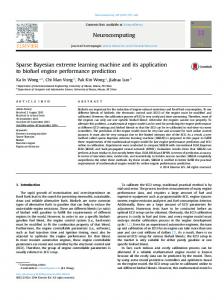
(b) λ = 1. Fig. 1. Distributions of Tdiff obtained by the regularized ELM with and without LOO cross validation.

(a) Regularized ELM with LOO.

(b) Regularized ELM without LOO.

Fig. 2. Misclassification comparisons between regularized ELM with and without LOO cross validation.

i.e., L < N and L ≥ N, whereas the method proposed in Heeswijk and Miche (2015) has the disadvantage in the computation cost when L ≥ N. As pointed out in the above, computations of the HATr matrix and the optimal output weight matrix βˆ are irrelevant with V when L ≥ N. Thus, instead of computing the singular value decomposition (SVD) on H in Heeswijk and Miche (2015), we directly compute the eigendecomposition on HHT . To further reduce the computational burden of the cross validation strategy in conventional LOO (Heeswijk & Miche, 2015), some tricks can also be used for fast calculation. Besides (Heeswijk & Miche, 2015), it is also worth pointing out that the LOO based cross validation is widely used in the pruning based ELM algorithms, such as the optimally pruned ELM (OP-ELM) (Miche et al., 2010) and the Tikhonov regularization based OP-ELM (TROP-ELM) (Miche, Heeswijk, Bas, Simula, & Lendasse, 2011). In contrast to our proposed method, the OP-ELM is devoted to using the LOO criterion for the best hidden neuron selections. During the pruning process in OP-ELM, the multiresponse sparse regression (MRSR) method is first employed to rank all the hidden neurons in the basic ELM network and then the LOO cross validation error is used to select the best number of neurons. As an extension of OP-ELM, the TROP-ELM focuses on the best hidden neuron pruning for the regularized ELM algorithm. The least square angle regression (LARS) with the ℓ1 penalty is adopted for hidden neuron ranking in the regularized ELM. Although the LOO method has been adopted in all these algorithms, it is noted that the calculation is different and our method has the lowest

computational complexity. Furthermore, the pruning based ELM is dedicated to finding the best hidden neurons by searching from a large number of initial candidates, whereas ours focuses on optimizing the regularization coefficient. As ELM performs classification through finding the largest entry of the output vector for a query input, one can expect that optimal regularized ELM can generate the maximal decision boundary for classification. This can be further explained by the actual ELM output. In fact, the difference between the first and second largest entries for each output vector can reflect the decision boundary to some extent whenever ELM employs the one-against-all (OAA) label-coding (Cao et al., 2012). For the sake of clarity, we denote the difference as Tdiff = of − os , where of and os represent the first and second largest entries in the ELM output vector, respectively. In general, the larger the value of Tdiff is, the better the classification boundary tends to be. Note that Tdiff has been first applied as a criterion in Luo and Zhang (2014) for noisy image partition, and it has shown that clean input images are prone to have large Tdiff in the ELM network output vector. To show the validity of the above analysis, experiments are conducted on the AR face dataset (Martinez & Benavente, 1998), which includes 700 training samples and 700 testing samples from 100 categories. The optimal regularization parameter is searched within {e−5 , e−4 , . . . , e5 } using the LOO error, while for the general regularized ELM, λ = 0.2 and λ = 1 are used. Figs. 1 and 2 depict the distributions of Tdiff and the number of samples with

96

J. Cao et al. / Neural Networks 81 (2016) 91–102

(a) Accuracy.

(b) Testing time. Fig. 3. Recognition accuracy and testing time w.r.t. different sub-dictionary sizes.

different values of Tdiff obtained by the regularized ELM with and without using the LOO cross validation approach, respectively. It is apparent that LOO error based optimal regularized ELM generally has larger Tdiff than the two regularized ELM with manually chosen regularization parameters. Moreover, the misclassification number counted in Fig. 2 also demonstrates that the optimal regularized ELM can achieve better performance. 3.2. Adaptive sparse representation by ELM As mentioned earlier, the ELM classifier has the advantage of fast model training speed, while SRC shows superiority in handling noisy image classifications. The hybrid classifier ELM-SRC, which has complementary strengths in learning speed and recognition accuracy, has been implemented for image classification (Cao, Zhao, Lai, Ong et al., 2015; Luo & Zhang, 2014). In the cascaded classifier, images with low noise are dealt with ELM and for those noisy images, SRC is adopted. Image partition through the Tdiff in an ELM output vector is one of the important contributions in ELMSRC. In fact, it is normal to view ELM misclassified images as noisy images, and in general ELM misclassification is caused by noisy images. In this sense, the noisy image partition is to estimate the ELM misclassified images. Motivated by this, the absolute difference between the first two largest elements in an ELM output vector could be a discriminative criterion. If the difference is larger than a predefined threshold, then the corresponding image is viewed as a clean image, otherwise, the associated image is reclassified by the SRC classifier. Such a strategy has shown promise in face recognition and landmark recognition (Cao, Zhao, Lai, Ong et al., 2015; Luo & Zhang, 2014). However, these only consider the information of the first two largest entries in the ELM output and the classification results tend to be less accurate than a SRC classifier. What is more, in the SRC classification stage, an universal and over-complete dictionary is used to represent the query image and thus lacks adaptability. It has already been pointed out that sparse representation over a highly redundant dictionary is potentially unstable due to the negative effects of uncorrelated classes (Timofte & Gool, 2014; Zhang, Yang, & Feng, 2011). In other words, the query image can be better classified by the sub-dictionary containing similar classes rather than the entire dictionary. In order to fully exploit the information of an ELM output and adaptively select the correlated classes for the query image in the dictionary, we further take the first k largest elements in the ELM output into consideration due to the fact that the uncorrelated classes tend to have a small response in an ELM output. More precisely, for a query image y assigned to SRC, the

indexes of the k largest elements in the output vector are recorded. Then, the atoms in the training dataset with the same labels as the k largest entries are picked up to construct a sub-dictionary for sparse representation adaptively. The compact sub-dictionary is expressed as A∗y = [Am(1) , Am(2) , . . . , Am(k) ], where m(i) ∈ {1, 2, . . . , m} is one of the indexes of the k largest entries and Am(i) denotes all the training samples belonging to the m(i)-th class. Hence, instead of calculating the sparse representation coefficients over all the training samples, we solve the following problem, xˆ = arg min ∥A∗y x − y∥22 + τ ∥x∥1 x

(17)

where τ is the regularization parameter for SRC. From (17), we can see that it actually forces the sparse representation coefficients of the query image over the other irrelevant sub-dictionaries to be zero. In other words, the adaptive sub-dictionary selection by ELM will naturally ensure the sparsity of the representation coefficients. To show the effectiveness of the proposed adaptive sub-dictionary coding approach, Fig. 3 presents the comparisons on the recognition accuracy (Fig. 3(a)) and average testing time per image (Fig. 3(b)) with respect to (w.r.t.) different sub-dictionary sizes of the AR face database. It is apparent that using the overall samples (k = 100 in Fig. 3) as the dictionary for sparse representation not only degrades the recognition performance but also increases the computational complexity. When k = 60 which means the sub-dictionary is constructed using atoms of the same labels to indexes of the 60 largest entries in the estimated output vector, the EA-SRC algorithm reaches the highest recognition accuracy. Utilizing the LOO error optimization based regularized ELM and the adaptive sub-dictionary construction approach for sparse representation, the developed EA-SRC classifier is able to enhance the classification accuracy as well as reduce the computational complexity for image classification. There are two general steps in the proposed EA-SRC algorithm. In the first step, for a given training database and a candidate set of the regularization parameter [λmin , λmax ], the SLFN is trained with the regularized ELM algorithm and the optimal regularization parameter λopt is derived by the LOO cross validation approach. In the meantime, the output weight matrix corresponding to the optimal regularized ELM is also computed through (14) or (16). In the second step, for each query image, the output vector is calculated using the trained SLFN by the regularized ELM. The criterion that measures the difference between the first and the second largest entries of the output vector is employed for image partition. As analyzed in Luo and Zhang (2014), if the actual network output obtained

J. Cao et al. / Neural Networks 81 (2016) 91–102

by the regularized ELM is an outlier of the desired one, it may imply misclassification and then the image is considered to contain high noise. For these images, ELM generally fails in recognition and the SRC approach should be adopted (Luo & Zhang, 2014). A large Tdiff = of − os means the image tends to contain less noise than the one with a small Tdiff. Thus, the image partition can be performed by comparing Tdiff to an appropriately chosen positive threshold σ . If Tdiff > σ , the classification is based on the ELM output. Otherwise, the query image will be fed to SRC. In this case, the sub-dictionary A∗y for sparse representation is first constructed for the image by collecting the atoms with the same labels to indexes of the k largest entries in the output vector of ELM. The sparse coefficient is then computed via (17) and the classification is performed by finding the minimal residual given by (9). In summary, a detailed pseudo-code of the proposed EA-SRC classifier is given in Algorithm 4. Algorithm 4: Proposed EA-SRC Classifier. Input

: A training database A with m classes, a query image y, a candidate set of ELM regularization parameter λ [λmin , λmax ], τ > 0, threshold σ . Output : Class label of y

3

Randomly generate hidden node parameters (wi , bi ), i = 1, 2, . . . , L. Calculate H(w1 , . . . , wL , x1 , . . . , xN , b1 , . . . , bL ). Use algorithm 3 to find the optimal λopt and give the corresponding

4

output weight matrix βˆ . Calculate the output o of ELM with respect to y via

1

2

5 6

o = H(w1 , . . . , wL , y, b1 , . . . , bL )βˆ ; if of − os > σ then Label(y) = arg max(o); d∈[1,...,m]

7 8 9 10 11 12 13 14 15 16

end else Find the indexes of k largest entries in o; Get the adaptive sub-dictionary A∗y for the image y;

solve xˆ = arg minx ∥A∗y x − y∥22 + τ ∥x∥1 ; for d ∈ {m(1), . . . , m(k)} do Find Ad and δd (ˆx); Calculate the residuals rd (y) = ∥y − Ad δd (ˆx)∥22 ; end Label(y) = arg min rd (y) d∈{m(1),...,m(k)}

17

end

4. Experimental results This section presents the experimental results on image classification problems with the proposed EA-SRC classifier. Experiments are conducted on three benchmark databases, including the USPS handwritten digits database, the Nanyang Technological University campus landmark database (NTU) and the AR face database. A brief specification of the three databases is given in the following.

• The USPS digits database consists of handwritten digits from 0 to 9 with a total of 11,000 samples collected from disjoint writers. • The NTU database contains 4156 landmark images belonging to 50 categories, which are captured in NTU campus, including buildings, structures, places of interests, etc. • The AR face database includes 700 training and 700 testing samples, which belong to 100 individuals.

97

Table 1 Classification results by different classifiers. Classifiers

ELM OP-ELM SRC ELM-SRC EA-SRC

Accuracy (%)

94.89 96.24 97.69 97.47 97.73

Time (s) Training

Testing

3.82 6.77 – 3.82 4.81

0.0007 0.0021 0.2752 0.0074 0.0043

The performance is compared with the regularized ELM with manually chosen regularization parameters (Huang, 2015), OPELM (Miche et al., 2010), SRC classifier (Wright, Yang et al., 2009), and ELM-SRC classifier (Cao, Zhao, Lai, Ong et al., 2015; Luo & Zhang, 2014). In the developed EA-SRC algorithm, the optimal regularization parameter is searched within {e−5 , e−4 , . . . , e5 } using the LOO cross validation based on the minimum MSEPRESS . Experiments are carried out in the Matlab R2014a on a PC with a Intel(R) Core(TM) i3-3240 processor with a speed of 3.40 GHz. The Matlab code of EA-SRC is available at http://www.escience.cn/people/Jiuwencao/Achievements.html. 4.1. Experiment on the USPS handwritten digit classification Each digit sample in the USPS database is a grayscale image of 16 × 16 pixels with an intensity from 0 to 255. Some handwritten digit samples are shown in Fig. 4. Here, the concatenated columns of the original image are directly used as the features. Since data normalization is necessary for most of classifiers, here the features are scaled into the range [0,1] for ELM classifier, whereas for SRC classifier each feature is normalized to have a unit ℓ2 -norm. We randomly choose 700 images per digit for training and use the remaining 400 images for testing, thus leading to the partition of whole database with 7000 training samples and 4000 testing samples. The number of hidden nodes for ELM and OP-ELM is set to be 1500, the regularization parameter τ for SRC is set to 0.1. Following Luo and Zhang (2014), the Matlab function ‘‘SolveHomotopy_CBM_std’’ (available for download from http://www.eecs.berkeley.edu/~yang/software/l1benchmark/) is adopted to calculate the sparse coefficients with the non-negative constrains. In order to further validate the effectiveness of the adaptive subdictionary selection strategy by ELM and also give an empirical study on the choice of parameter pair (σ , k), Fig. 5 shows the training and testing accuracies of EA-SRC with respect to various combinations of σ and k under the assumption that the samples classified by SRC procedure give correct class labels. Note that we use this assumption such that, once the ELM classifier is obtained, the only parameters that influence the accuracy of EA-ELM are σ and k. It can be seen that both of the training and testing accuracies improve with the increase of σ and k. When σ is fixed, the accuracy does not have much gain when k is larger than 4, thus validating the effectiveness of the adaptive sub-dictionary selection strategy. Considering that a larger σ or k will lead to more computational complexity, the choice of parameter pair (σ , k) should make a compromise between accuracy and computational complexity. Based on the above discussion, we set σ and k to be 0.3 and 4, respectively. Table 1 shows the experimental results of the handwritten digit classification with ELM, OP-ELM, SRC and ELM-SRC and EA-SRC, respectively. As one can see, our proposed EA-SRC gives the best testing accuracy. By adopting LOO error based optimization for the ELM regularization parameter, the training time only increases by 1s when ten extra parameters are searched (compared to the original ELM). Therefore, we argue that the proposed LOO error based optimization is an efficient solution for optimizing

98

J. Cao et al. / Neural Networks 81 (2016) 91–102

Fig. 4. Some handwritten digit samples.

(a) Training.

(b) Testing. Fig. 5. Training and testing accuracies of EA-SRC with respect to various combinations of σ and k.

the regularization parameter of ELM. As for the testing time, our proposed EA-SRC is much faster than ELM-SRC, which is attributed to the adaptive sub-dictionary selection strategy and the regularization parameter optimization for ELM. In addition, the testing speed of the proposed EA-SRC method is somewhat comparable to that of ELM and OP-ELM. Thus, we can come to the conclusion that the EA-SRC method achieves the best performance in terms of accuracy and testing time. Fig. 6 provides an illustration of the superiority of the proposed EA-SRC. It can be seen that, given the testing digit ‘‘0’’ which belongs to the tenth class, the difference of the first and second largest entries of the actual ELM output is less than the threshold σ . Consequently, SRC with an adaptive sub-dictionary determined by candidate class labels {2, 4, 7, 10} is used for further classification. As shown in Fig. 6(c), one can see that if we use SRC classifier without an adaptive sub-dictionary selection strategy, the wrong class label 4, which corresponds to the minimum residual, will be assigned to the query image. However, with the help of an adaptive sub-dictionary selection strategy, the correct class label is given and the gap between the first two smallest residuals is larger than that without adaptive sub-dictionary selection strategy. In fact, the performance of the SRC method can be affected by the irrelevant samples in the dictionary. By incorporating the ELM classifier and the adaptive sub-dictionary selection strategy, our proposed EA-SRC method can reduce this influence while improving computation cost. This explains why our proposed method can outperform SRC. 4.2. Experiment on the NTU landmark recognition Landmark cognition has recently been widely researched due to the popularity and development of smart terminals in the past decade (Chen & Yap, 2014). Recognition accuracy and computational complexity are the two vital aspects for a landmark recognition system. Besides the most frequently used support vector machine (SVM), we have recently explored the SRC

algorithm in Cao, Zhao, Lai, Chen et al. (2015). To further reduce the computational cost of the sparse coefficient calculation, we employed the ELM-SRC approach to shorten the overall testing time in Cao, Zhao, Lai, Ong et al. (2015). In this section, we evaluate the performance of the proposed EA-SRC classifier on the NTU campus landmark database. In the experiment, 3533 landmark images are used for training and dictionary construction while the remaining 623 samples are used for testing. The bagof-words (BoW) histogram representation approach is utilized to reduce the extracted dense scale-invariant feature transform (SIFT) features, and 200 features are used for experiments. For a sparse coefficient calculation, the non-negative homotopy method (Yang et al., 2010), which is not sensitive to the training data scales, is adopted for SRC, ELM-SRC, and EA-SRC. In this experiment, the threshold σ and the number of largest entries k are tested on the grid [0.1 : 0.1 : 1] and [5 : 5 : 30] respectively to show the variations of recognition rate on different noisy image partitions and different sub-dictionary sizes. For each paired parameters (σ , k), 50 independent trials of experiments are conducted and the average recognition accuracy as well as the testing time is reported. Fig. 7 plots the recognition accuracy of the proposed EA-SRC with respect to different thresholds σ and different number k. As shown in the figure, the recognition accuracy derived by EA-SRC is generally higher than 91% and lower than 93%. For a fixed size k of the sub-dictionary, the EASRC classifier achieves the best recognition performance when the threshold is around σ = 0.3 and σ = 0.4. The recognition accuracy is relatively stable when the threshold σ and the size of the sub-dictionary k are picked up in the regions σ ∈ [0.3, 1] and k ∈ [15, 30]. Computational complexity is another critical factor for landmark recognition. Fig. 8 depicts the speedups of the proposed EA-SRC algorithm with respect to the SRC algorithm in different thresholds σ and different number k of largest entries. The speedup is the ratio between the average testing time per image costed by SRC and EA-SRC. It is apparent that EA-SRC has a lower computational complexity in the testing phase for all different parameter combinations of the threshold σ and the size

J. Cao et al. / Neural Networks 81 (2016) 91–102

(a) Testing digit ‘‘0’’.

99

(b) Actual and desired ELM output.

(c) SRC residuals without adaptive sub-dictionary selection.

(d) SRC residuals with adaptive sub-dictionary selection.

Fig. 6. An illustration of the proposed EA-SRC method. Table 2 Performance comparisons on the NTU landmark database. Classifier

Accuracy (%) Testing time (s)

ELM

78.6 0.0014

OP-ELM

82.04 0.0084

SVM

83.52 0.0441

Homotopy

SpaRSA

FastLaplace

SRC

ELM-SRC

EA-SRC

SRC

ELM-SRC

EA-SRC

SRC

ELM-SRC

EA-SRC

91.84 0.4758

91.65 0.1187

93.02 0.0482

89 1.587

87.21 1.198

91.56 0.0127

89.41 2.914

87.58 1.089

91.28 0.0215

of sub-dictionary k used in the experiment. For certain cases, the speedup obtained by EA-SRC is higher than 36. The recognition performance comparisons on the landmark database are reported in Table 2. In this table, we compare EA-SRC with the original ELM, OP-ELM, SVM, ELM-SRC, and SRC algorithm on recognition accuracy and average testing per image, respectively. In the meantime, for EA-SRC, ELM-SRC, and SRC, we test the landmark recognition performance on three representative sparse coefficient estimation algorithms, namely, the non-negative homotopy method (Yang et al., 2010), the SpaRSA approach (Wright, Nowak et al., 2009) and the fast Laplace algorithm (FastLaplace) (Babacan et al., 2010), respectively. The regularization coefficient in SpaRSA is set to be 0.5. Following the analyses in above paragraph, the threshold σ for noisy image selection is set to be 0.3 and the number of largest entries k controlling the scale of the sub-dictionary is set to be 20 for all SRC based algorithms in this experiment. As shown in the table, ELM

has the shortest testing time amongst all compared algorithms but also suffers the lowest recognition rate. OP-ELM performs slightly better than ELM, but worse than the rest algorithms. For all SRC-associated classifiers, the proposed EA-SRC consistently provides better recognition performance than SRC and ELM-SRC correspondingly (as highlighted in bold in Table 2). What is more, with the same sparse coefficient estimator, the average testing time per image spent by EA-SRC is far less than that used by ELM-SRC and SRC. In addition, EA-SRC achieves more than 14% and 9% improvements over the original ELM and the popular SVM when using the non-negative homotopy method, while for the SpaRSA approach and the fast Laplace algorithm, the enhancements obtained by EA-SRC are higher than 12% and 8%, 12% and 7%, respectively. It is also worth pointing out that the presented EA-SRC method with the non-negative homotopy algorithm has a comparable testing time to SVM while SpaRSA and FastLaplace, EA-SRC have a faster testing speed than SVM.

100

J. Cao et al. / Neural Networks 81 (2016) 91–102

Fig. 7. Recognition accuracy of EA-SRC w.r.t. different thresholds σ and different number k of largest entries. Fig. 9. Recognition performance on different number of hidden nodes in ELM. Table 3 Comparisons of recognition accuracies (%) on the AR face database. Classifier

ELM SRC ELM-SRC EA-SRC

Fig. 8. Speedups of EA-SRC to SRC w.r.t. different thresholds σ and different number k of largest entries in the landmark database.

To validate the effectiveness of using the LOO error based regularization parameter optimization in ELM, we compare the recognition performance with different manually choosing λ on the landmark database. For ELM-LOO, the regularization parameter λ is searched within {e−5 , e−4 , . . . , e5 }. Six different regularization parameters, namely, λ = {0.05, 0.1, 0.3, 0.5, 0.7, 0.9} are tested as the manually chosen parameter in the regularized ELM. The recognition accuracies are collected for a number of hidden nodes varying from 500 to 1500. Using the LOO error approach, ELMLOO achieves the best performance for λ = e−3 , which is the optimal regularization parameter derived by the minimal LOO error. The recognition accuracies of the used ELM-LOO and ELM with different manually chosen regularization parameters with different hidden nodes are reported in Fig. 9. It is obvious that the LOO cross validation approach is able to find the optimal regularization parameter in ELM and ensure the best recognition accuracy. For manually chosen λ, the recognition performance is improving when the regularization parameter keeps increasing. However, the enhancement in recognition accuracy is decreasing, as reflected in the figure. 4.3. Experiment on the AR face recognition For the AR face database, the training and testing samples are fixed in our experiments. The AR images are cropped to dimension 60 × 43 and converted to grayscale. We directly work on the lower dimensional spaces and use the eigenfaces as the face features. Five different dimensional features {100, 150, 200, 250, 300} are tested. The ℓ1 -regularized least square problem solver (known

Dimensionality 100

150

200

250

300

83.57 89.42 89.57 90.93

85.14 91.57 91.71 92.79

85.57 92.57 92.43 94.07

86.14 93.14 93.00 94.21

86.42 93.57 93.43 94.74

as the Matlab function ‘‘l1_ls’’ (the Matlab code is available at http://web.stanford.edu/~boyd/l1_ls/) is adopted for sparse coefficient calculation in SRC, ELM-SRC, and EA-SRC. The number of hidden nodes for ELM is set to be 1000. In this experiment, we select σ = 0.1 as the threshold for noisy image partition in ELM-SRC and EA-SRC. This is based on the analysis given in Luo and Zhang (2014) that when Tdiff ∈ [0, 0.1], around half of these images are misclassified and when σ = 0.5, almost all the misclassified images can be picked out. Fig. 2(a) also verifies the statement. In addition, a large threshold σ generally provides a high recognition rate in ELM-SRC and EA-SRC classifiers but the computational complexity also increases as more image samples have been assigned to the time-consuming SRC. In the proposed EA-SRC, atoms in the training database with the same label as indexes, corresponding to k = 50 largest entries in the output vector, are adaptively picked up to construct the sub-dictionary for each query image. Table 3 lists recognition accuracies in the AR database. As one can see, EA-SRC consistently improves the recognition performance over the rest three classifiers for all five different eigenfaces. Compared to the regularized ELM, increments of recognition rate obtained by EA-SRC are more than 7%, while comparing with SRC and ELM-SRC, EA-SRC achieves more than a 1% improvement in the recognition accuracy for all five different eigenfaces. To compare the computational complexity, we collect the average testing time. There is no doubt that the regularized ELM wins with the shortest recognition time. However, due to its low recognition accuracy, we will only focus on the computational comparisons of SRC based classifiers, namely, SRC, ELM-SRC, and the proposed EA-SRC. Fig. 10(a) plots the curves of average testing time per image and Fig. 10(b) depicts the speedups of ELM-SRC and the proposed EA-SRC w.r.t. SRC, respectively. As shown in Fig. 10(a), SRC spends more than 0.6s (second) per sample for sparse coefficient calculation and image recognition when the dimension of eigenface feature is 100. The testing time keeps increasing when the dimension of the eigenface feature increases, and reaches more than 1s per image when the dimension of

J. Cao et al. / Neural Networks 81 (2016) 91–102

(a) Testing time.

101

(b) Speedup. Fig. 10. (a) Average time per image costed by SRC, ELM-SRC, and EA-SRC; (b) Speedup of ELM-SRC and EA-SRC w.r.t. SRC.

Fig. 11. Performance comparisons on AR face database using two activation functions with a different number of hidden nodes.

eigenface feature is 300. Incorporating ELM into SRC indeed reduce the computational complexity for ELM-SRC. However, the testing time per image costed by ELM-SRC is still around 0.4 s or longer for high dimensional eigenfaces. Thanks to adopting the adaptive subdictionary selection strategy for sparse representation, the testing time per image from the developed EA-SRC method reduces to around 0.05 s for all five different eigenface features. Compared to SRC, the speedup of EA-SRC is more than 10 for all five different eigenface features and is as high as 21 when the dimension of feature is 300. The affections of hidden neuron activation function and number of hidden nodes are also studied in this experiment. We test the classification accuracy on the AR face database using 11 different numbers of hidden nodes ranging from 500 to 1500 with two popular nonlinear activation functions, namely, the sigmoid function g (x) = 1+1e−x and the hyperbolic tangent function g (x) = sinh(x) . cosh(x)

In this experiment, the eigenface with 200 features is used for face image representation and the threshold in the EA-SRC method is set to δ = 0.1. The performance of the EA-SRC algorithm is compared with the conventional ELM for these two functions. Fig. 11 plots the classification accuracy comparisons, where the legends ‘‘ELM(s)’’, ‘‘ELM(t)’’, ‘‘EA-SRC(s)’’ and ‘‘ELM-SRC(t)’’ denote the ELM and the proposed EA-SRC algorithm using the sigmoid and hyperbolic tangent functions, respectively. EA-SRC method has better performance than ELM for all tested activation functions

and hidden nodes. In addition, it can be seen from the figure that EA-SRC has a consistent performance in classification accuracy for both two activation functions when using different number of hidden nodes. The variation among the number of hidden nodes and the two functions is small. For ELM, using the hyperbolic tangent function generally achieves a higher classification rate than using the sigmoid function. Using the same experimental parameter settings as the AR face database given in Timofte and Gool (2014), we also compare the recognition performance to several state-of-the-art approaches in this section, including the weighted collaborative representation classifier (WCRC) (Timofte & Gool, 2014), the adaptive weighted collaborative classifier (AWCRC) (Timofte & Gool, 2014), the iterative nearest neighbors classifier (INNC) (Timofte & Gool, 2012), the collaborative representations (CR) with regularized least squares (CRC-RLS) (Zhang et al., 2011), the standard linear support vector machines (LSVM) classifier as well as the OP-ELM algorithm. The results are obtained using 300 eigenface features. Table 4 lists the recognition accuracy for all these algorithms. As we can see, EASRC achieves the highest recognition accuracy 94.74% on the AR face database, which is 1.02%, 1.62%, 1.02%, 15.2%, 0.98%, 10.24%, 8.04% higher than WCRC (Timofte & Gool, 2014), AWCRC (Timofte & Gool, 2014), INNC (Timofte & Gool, 2012), CRC-RLS (Zhang et al., 2011), LSVM and OP-ELM, respectively. 5. Conclusion In this paper, we developed an EA-SRC image classifier based on the regularized ELM with an optimal regularization parameter and the SRC classifier with an adaptive sub-dictionary selection strategy. The LOO cross validation approach has been adopted to optimize the regularization parameter of ELM and thus the classification hyperplane has been optimized. Moreover, for each query image, an adaptive sub-dictionary selection strategy that exploits correlations of the testing image and the training database has been proposed for sparse representation dictionary construction. Experimental results from three popular databases: USPS digit database, NTU landmark database and AR face database, are conducted to show the overall efficiency and effectiveness of the proposed EA-SRC over ELM, OP-ELM, SRC, ELM-SRC and several state-of-the-art classifiers. Acknowledgments This work was supported by the NNSF of China (61503104, 61573123) and Zhejiang Provincial Natural Science Foundation of China (LY15F030017).

102

J. Cao et al. / Neural Networks 81 (2016) 91–102

Table 4 Comparisons on the AR face database w.r.t. state-of-the-art classifiers. Classifier

WCRC (Timofte & Gool, 2014)

AWCRC (Timofte & Gool, 2014)

INNC (Timofte & Gool, 2012)

CRC-RLS (Zhang et al., 2011)

LSVM

OP-ELM

EA-SRC

Accuracy

93.72

93.12

79.54

93.76

84.5

86.7

94.74

References Babacan, S., Molina, R., & Katsaggelos, A. (2010). Bayesian compressive sensing using laplace priors. IEEE Transactions on Image Processing, 19, 53–63. Bai, Z., Huang, G.-B., Wang, D., Wang, H., & Westover, M. (2014). Sparse extreme learning machine for classification. IEEE Transactions on Cybernetics, 44, 1858–1870. Bai, T., Li, Y.-F., & Zhou, X. (2015). Learning local appearances with sparse representation for robust and fast visual tracking. IEEE Transactions on Cybernetics, 45, 663–675. Cao, J., Chen, T., & Fan, J. (2016). Landmark recognition with compact bow histogram and ensemble ELM. Multimedia Tools and Applications, 75, 2839–2857. Cao, J., & Lin, Z. (2014). Bayesian signal detection with compressed measurements. Information Sciences, 289, 241–253. Cao, J., & Lin, Z. (2015a). Extreme learning machines on high dimensional and large data applications: A survey. Mathematical Problems in Engineering, 2015, 1–12. Cao, J., & Lin, Z. (2015b). Performance bound of multiple hypotheses classification in compressed sensing. In IEEE international symposium on circuits and systems. ISCAS (pp. 433–436). Cao, J., Lin, Z., Huang, G.-B., & Liu, N. (2012). Voting based extreme learning machines. Information Sciences, 185, 66–77. Cao, J., Zhao, Y., Lai, X., Chen, T., Liu, N., Mirza, B., & Lin, Z. (2015). Landmark recognition via sparse representation. In 2015 IEEE international conference on digital signal processing. DSP2015 (pp. 1030–1034). Cao, J., Zhao, Y., Lai, X., Ong, M., Yin, C., Koh, Z., & Liu, N. (2015). Landmark recognition with sparse representation classification and extreme learning machine. Journal of the Franklin Institute, 352, 4528–4545. Chen, D., & Girod, B. (2015). A hybrid mobile visual search system with compact global signatures. IEEE Transactions on Multimedia, 17, 1019–1030. Chen, T., & Yap, K. H. (2014). Discriminative bow framework for mobile landmark recognition. IEEE Transactions on Cybernetics, 44, 695–706. Czarnecki, W. (2015). Weighted tanimoto extreme learning machine with case study in drug discovery. IEEE Computational Intelligence Magazine, 10, 19–29. Deng, W.-Y., Zheng, Q.-H., & Wang, Z.-M. (2014). Cross-person activity recognition using reduced kernel extreme learning machine. Neural Networks, 53, 1–7. Donoho, D. (2006). Compressed sensing. IEEE Transactions on Information Theory, 52, 1289–1306. Du, X., & Cheng, L. (2014). Three stochastic measurement schemes for direction-ofarrival estimation using compressed sensing method. Multidimensional Systems and Signal Processing, 25, 621–636. España-Boquera, S., Castro-Bleda, M., Gorbe-Moya, J., & Zamora-Martinez, F. (2011). Improving offline handwritten text recognition with hybrid HMM/ANN models. IEEE Transactions on Pattern Analysis and Machine Intelligence, 33, 767–779. Ghofrani, S. (2015). Matching pursuit decomposition for high-resolution direction of arrival. Multidimensional Systems and Signal Processing, 26, 693–716. Han, X.-H., Chen, Y.-W., & Xu, G. (2015). High-order statistics of weber local descriptors for image representation. IEEE Transactions on Cybernetics, 45, 1180–1193. Heeswijk, M., & Miche, Y. (2015). Binary/ternary extreme learning machines. Neurocomputing, 149, 187–197. Huang, G.-B. (2015). What are extreme learning machines? filling the gap between Frank Rosenblatt’s dream and John von Neumann’s puzzle. Cognitive Computation, 7, 263–278. Huang, G., Huang, G.-B., Song, S., & You, K. (2015). Trends in extreme learning machines: A review. Neural Networks, 61, 32–48. Huang, G., Liu, T., Yang, Y., Lin, Z., Song, S., & Wu, C. (2015). Discriminative clustering via extreme learning machine. Neural Networks, 61, 1–8. Huang, G.-B., Zhu, Q.-Y., & Siew, C.-K. (2006). Extreme learning machine: Theory and applications. Neurocomputing, 70, 489–501. Iosifidis, A., Tefas, A., & Pitas, I. (2016). Graph embedded extreme learning machine. IEEE Transactions on Cybernetics, 46(1), 311–324. Li, S., You, Z.-H., Guo, H., Luo, X., & Zhao, Z.-Q. (2016). Inverse-free extreme learning machine with optimal information updating. IEEE Transactions on Cybernetics, 46(5), 1229–1241.

Liu, H., Guo, D., & Sun, F. (2016). Object recognition using tactile measurements: Kernel sparse coding methods. IEEE Transactions on Instrumentation and Measurement, 65, 656–665. Liu, H., Liu, Y., & Sun, F. (2015). Robust exemplar extraction using structured sparse coding. IEEE Transactions on Neural Networks and Learning Systems, 26, 1816–1821. Luo, J., Vong, C.-M., & Wong, P.-K. (2014). Sparse Bayesian extreme learning machine for multi-classification. IEEE Transactions on Neural Networks and Learning Systems, 25, 836–843. Luo, M., & Zhang, K. (2014). A hybrid approach combining extreme learning machine and sparse representation for image classification. Engineering Applications of Artificial Intelligence, 27, 228–235. Martinez, A., & Benavente, R. (1998). The AR face database, Tech. Rep. 24, CVC Tech. Report. Miche, Y., Heeswijk, M., Bas, P., Simula, O., & Lendasse, A. (2011). TROPELM: A double-regularized elm using lars and tikhonov regularization. Neurocomputing, 74, 2413–2421. Miche, Y., Sorjamaa, A., Bas, P., Simula, O., Jutten, C., & Lendasse, A. (2010). OP-ELM: Optimally pruned extreme learning machine. Neurocomputing, 21, 158–162. Myers, R. (1990). Classical and modern regression with applications. Duxbury. Olshausen, B., & Field, D. (1996). Emergency of simple-cell receptive field properties by learning a sparse coding for natural images. Nature, 381, 607–609. Pao, Y.-H., Park, G., & Sobajic, D. (1994). Learning and generalization characteristics of the random vector functional-link net. Neurocomputing, 6, 163–180. Pao, Y.-H., & Takefuji, Y. (1992). Functional-link net computing: theory, system architecture, and functionalities. Computer, 25, 76–79. Timofte, R., & Gool, V. (2012). Iterative nearest neighbors for classification and dimensionality reduction. In IEEE conference on computer vision and pattern recognition. CVPR (pp. 2456–2463). Timofte, R., & Gool, V. (2014). Adaptive and weighted collaborative representations for image classification. Pattern Recognition Letters, 43, 127–135. Vinje, W., & Gallant, J. (2000). Sparse coding and decorrelation in primary visual cortex during natural vision. Science, 287, 1273–1276. Wang, J., Lu, C., Wang, M., Li, P., Yan, S., & Hu, X. (2014). Robust face recognition via adaptive sparse representation. IEEE Transactions on Cybernetics, 44, 2368–2378. Wright, S., Nowak, R., & Figueiredo, M. (2009). Sparse reconstruction by separable approximate. IEEE Transactions on Signal Processing, 57, 2479–2493. Wright, J., Yang, A., Ganesh, A., Sastry, S., & Ma, Y. (2009). Robust face recognition via sparse representation. IEEE Transactions on Pattern Analysis and Machine Intelligence, 31, 210–227. Yang, A., Sastry, S., Ganesh, A., & Ma, Y. (2010). Fast ℓ1 -minimization algorithms and an application in robust face recognition: A review. In 2010 17th IEEE international conference on image processing. ICIP (pp. 1849–1852). http://dx.doi.org/10.1109/ICIP.2010.5651522. Yang, A., Zhou, Z., Balasubramanian, A., Sastry, S., & Ma, Y. (2013). Fast ℓ1 minimization algorithms for robust face recognition. IEEE Transactions on Image Processing, 22, 3234–3246. Yin, C., Cheng, Y., Chen, Y., Stark, B., & Zhong, S. (2015). Adaptive fractionalorder switching-type control method design for 3d fractional-order nonlinear systems. Nonlinear Dynamics, 82, 39–52. Yin, C., Chen, Y., & Zhong, S. (2014). Fractional-order sliding mode based extremum seeking control of a class of nonlinear system. Automatica, 50, 3173–3181. Zhang, K., & Luo, M. (2015). Outlier-robust extreme learning machine for regression problems. Neurocomputing, 151, 1519–1527. Zhang, L., Yang, M., & Feng, X. (2011). Sparse representation or collaborative representation: Which helps face recognition?. In IEEE international conference on computer vision. ICCV (pp. 471–478). Zhu, X., Li, X., & Zhang, S. (2016). Block-row sparse multiview multilabel learning for image classification. IEEE Transactions on Cybernetics, 46(2), 450–461.