humanoid robots, the sense of touch becomes even more important due to the ... to recognize a person, the process of identification is invisible for the human.
Face classification using touch with a humanoid robot hand Nicolas Sommer and Aude Billard Ecole Polytechnique Federale de Lausanne (EPFL) {n.sommer, aude.billard}@epfl.ch
Abstract—This paper presents an experiment in which the iCub humanoid robot learns to recognize faces through proprioceptive information. We take inspiration in the way blind people recognize people’s faces, i.e. through tactile exploration of the person’s face. The iCub robot’s tactile sensors are used to provide compliance in the hand motion so as to smoothly scan the facial features. The displacement of the fingers, as the robot explores the face, is used to build a model of the face using Hidden Markov Models. We show that the robot can successfully distinguish across the faces of a standard doll and the faces of three humanoid robots, the HOAP-3 robot, a Robota doll robot and MyDreamBaby, a commercial robotic doll. Keywords: face recognition, tactile sensing, humanoids, human-robot interaction.
I. I NTRODUCTION Recent progresses in tactile sensing offer a range of novel research directions in robotics, such as recognition of objects through texture [1] and safety during physical human-robot interaction [2]. In humanoid robots, the sense of touch becomes even more important due to the resemblance of these robots to humans and the fact that touch is an essential sense for humans. In this work, we explore ways in which this new modality can be used in combination with proprioception to identify people’s faces. Although computer vision is now an effective way for robots to recognize a person, the process of identification is invisible for the human. It is also very sensitive to illumination conditions and provides only partial information about texture and other individual specific facial features. We seek to provide robots with the ability to create a map of facial features through tactile exploration. This process mimics the way in which blind people build a representation of people’s faces. The task of classifying faces through proprioceptive information, using touch to guide the hand and finger motion across the faces, belongs to the broader range of surface and object recognition techniques. Various approaches have been proposed towards that goal. A series of recognition methods are based on local probing of the object, for instance by creating a tactile image of the contact between a grasped object and the gripper and differentiating between rough flat, edge, cylindrical and spherical contact shapes using a neural network [3]. Another local approach is to model the curvature of a surface at one point by using data from three differently oriented curves that are concurrent at the interest point and comparing the parameters of this local feature (normal direction and the two main curvatures) [4]. However, comparing a local feature is often not enough to distinguish between two complex objects. In [5], a bag-offeatures approach is applied to generate object histograms describing their local features along their length, with tactile information retrieved from several grasps at different positions. Moreover, once the learning completed, in order to minimize the required number of grasp actions, a new grasp location is chosen on the object by maximizing the expected information gain on the probabilistic belief
about the type of object. A hybrid approach uses both tactile and haptic information in [6] by completely modelling objects with 3D point clouds representations, systematically scanning the objects with grippers equipped with tactile sensor arrays, or by creating Self-Organizing Maps from few grasps with more complex robotic hands [7], [8]. In contrast to the methods reviewed previously, it might be preferable to continuously probe an object surface instead of discretely grasp or touch an object: humans do not release and grasp several times an object in order to recognize it by touch but rather follow the surface with their fingers. In [9], a tactile sensor array is moved around the surface of a convex-shaped object while passively rotating to follow the slope. The time-series of 2D pressure profiles are fed to several neural networks for classification after local PCA for feature extraction and dimensionality reduction. In another application, continuous probing is used to identify surfaces by mobile robots [10]: the probe uses an accelerometer attached near its tip in contact with the ground to collect data describing the surface on which the robot is moving. Classification is done by analysing selected features of the data from fixed time windows. From the perspective of using tactile data to drive compliant motions, [11] uses information from fingertip tactile sensors on a robotic hand to compliantly adapt the grasp of a selection of objects, by learning the non-linear correlation between finger position and tactile signature. Our work combines the notion of continuous exploration of the surface and the idea of compliant control introduced in these other works. Precisely, we use a) the tactile fingertips to introduce a compliant mechanism for the displacement of the fingers along the face and b) proprioceptive information, i.e. the position of the fingers during a motion, to classify the faces. In contrast with most of the previous works, this process does not require to probe iteratively different locations, or to build a precise 3D model of the face. Our approach rather relies on the essential characteristics of one continuous human-like motion across the face. II. T HE PROBING MECHANISM The goal of the experiment is to identify a face by touch. In order to do so, our humanoid robot - the iCub robot [12] - moves its hand in a vertical plane, while its fingers actively follow the curve of the face to track its shape1 .There are four faces to classify in this experiment (see Figure 1). The faces have been chosen because they all share similar basic features (eyes, mouth, roundness of the head), hence making the task to distinguish across their features more challenging: the traditional doll (Doll1) and the robotic doll (Doll2) have faces that are extremely similar from a tactile-view point, as the overall surface of the face and the distance across facial features are almost identical. Major differences lie in the shape of the mouth and nose 1 The
experiments are illustrated in a video with this paper.
(a) Doll1 (10x12cm)
(b) Doll2 (c) Robota (d) HOAP (MyDreamBaby, (plaster cast, (12x13cm) 9x12cm) 15x13cm)
Fig. 3: Front view scheme of hand trajectories and starting points – red dots – on HOAP. Each dot represents the center of the middle and index fingertips on the head, at the beginning of the motion.
Fig. 1: Faces to be sorted in the experiments(width x heigth)
of the two dolls. The face of the robot Robota is a scaled version of the Doll1 robot and again differs from the previous faces mainly through its overall size, as well as the relative proportion of the face covered by the eyes and nose. The face of HOAP-3 robot is the most distinctive of all four faces, because of its protruding forehead and its lack of a nose. A. iCub The iCub robot is a 53-DOFs humanoid robot whose arms are composed of 7 joints, plus 9-DOFs hands (see Figure 2). The 7 arm joints are used to achieve the vertical motion of the hand while one joint per finger is used to follow the face (sole index and middle finger are used in this experiment).
Fig. 4: The fingers follow the curve of the face. On the left, a wide angle describes the depression of the eyes and on the right, the nose bump yields a smaller angle.
experiments. The angular values of the finger joints are recorded during the experiment. Each motion lasts approximately between 7 and 10 seconds, depending on the size of the face. The ten recordings of these angular values form the dataset used in the learning phase. Data are gathered at a rate of 50Hz, resulting in 400 datapoints on average. C. Pressure control with tactile sensing
(a)
(b)
Fig. 2: Experimental set-up: a) The iCub robot moves slowly a finger over the face of Doll1 and captures an image of the face of the robot through proprioceptive measurement. b) The iCub’s hand is endowed with tactile sensors at the finger tips.
The goal of the experiment is to record the motion of the fingers while they stay in contact with the face. This is achieved through tactile pressure control. Our iCub robot is endowed with capacitive tactile sensors on its fingertips [13]. Each of these sensors is composed of 12 taxels tpf (i.e. tactile pixels), tpf ∈ [0, 255], with finger f = 1, 2 and taxel p = 1..12. The average pressure per finger sf is used here as the controlled variable for the pressure loop:
sf =
12 1 X p tf 12
(1)
p=1
B. Hand trajectory The hand is controlled so as to follow a predefined vertical line from the top to the bottom of the face, keeping a fixed orientation, palm facing the scanned head, pointing upwards, see Figure 4. The motion starts with the fingers at the level of the forehead and is stopped manually when the fingers reach the bottom of the face. For each face, this motion is repeated ten times: at each run, the hand is shifted horizontally so as to span homogeneously the whole width of the face (see Figure 3). These ten trajectories are used during the learning phase to create a model of the face (see Section III). During the motion, the index and middle fingers stay in contact with the face by means of a pressure loop (detailed in the next section). Since the ring and little fingers are coupled and cannot be controlled independently, they are not used in the experiment: they cannot follow two different profiles simultaneously. The spacing between the fingers (adduction/abduction) is fixed during all the
Note that the faces used in the experiments have been covered with aluminium foil because this enhances the response of the capacitive sensors and hence ensures better tactile pressure control (refer to Figure 4). A PD controller is implemented to follow a constant target pressure sˆf . This target pressure is manually adjusted so as to keep a contact with the face without damaging the fingers. Each finger f is thus controlled in current uf following: uf (sf , sˆf ) = κp (ˆ sf − sf ) − κd s˙ f where s˙f is the derivative of the total pressure at each finger, and κp ∈ < and κd ∈ < are the proportional and derivative coefficients2 . 2 In our implementation, the gains κ and κ are hand-tuned. Note that p d these gains operate on values of current, which are then mapped to torque commands for the motors.
III. FACE IDENTIFICATION
Raw data: first 6 middlefinger trajectories on Doll 2 20
15
10
5 0
1
2
3
4
5
6
Timestep (s) Pre−processsed data: first 6 middlefinger trajectories on Doll 2 0.2
0.1
dx2 dz
The raw data from the experiments are the angles θft,n , with f = 1..F fingers (F = 2, index and middle fingers), n = 1..N demonstrations and t = 1..T timesteps. These values depend heavily on the distance between the hand and the face: the same face profile yields different results if the face to identify is slightly moved away from iCub’s hand. A few pre-processing steps enable to get rid of this issue. First, we take the sinus of the angles in order to have a value linearly correlated with the distance between the hand and the face:
θ2 (deg)
A. Data pre-processing
0
−0.1
xt,n = sin(θft,n ) f
(2) −0.2
�
t,n T
0
This gives us the data set xf t=0 (see Figure 5). The remaining constant shift following from the hand being further away during another motion can be removed by simply taking the derivative of x with respect to z, the vertical coordinate.
20
40
60
80
100
120
140
z (Relative vertical coordinate index)
Fig. 6: Comparison between raw and pre-processed data on the first 4 middle finger motions recorded on Doll2.
differ depending on which part of the face is spanned by the finger (to recall, each of the trajectory is initialized at a different location along the width of the face). B. Learning algorithm
Fig. 5: Scheme of the finger probing system for one finger. The hand moves along the z axis. This linearised value is time dependent and the vertical velocity profile of the hand motion is not flat (the velocity is not exactly constant during the motion), we therefore re-sample the values according � g,n G to the Cartesian vertical coordinate z. The new dataset x ˜f g=0 , indexed by g, spans regularly the vertical axis z. The data points x ˜ are interpolated from x, with G the chosen number of sampled datapoints3 . The linearised profile is then differentiated with respect to z to obtain a set of data independent from the velocity of the hand during the motion:
( Dr =
d˜ xg,n f dz
=
x ˜g,n −x ˜g−1,n f f
)F,N,G (3)
∆z f =1,n=1,g=1
with r ∈ {Doll1, Doll2, Robota, HOAP }. The data is then de-noised using a lowess filter [14] – local regression using weighted linear least squares, here with a 1st degree polynomial model. These pre-processing steps yield data containing velocity profiles which describe the slope of the faces along two vertical lines described by the fingers. This information is sufficient to recreate the original face profiles – sectional views as in Figure 5 – by integrating the slope. The advantage of pre-processing the data is visible on Figure 6: while the raw trajectories are not aligned and vary in amplitude, the final data is much easier to compare. Note that the pre-processed curves are not perfectly aligned. This is expected, since the profiles 3G
was set to 140 points in the current implementation.
Due to the absence of reliable position measurement on our robot’s end effector, recognizing the essential characteristics of the motion of the finger when moving across the face (as opposed to recognizing the exact 3D trajectory) is preferable. To account for this inherent variability in the way we acquire data, we choose to encode the distribution of our datapoints through a densitybased representation. Such probabilistic encoding offers a flexibility that conventional data-driven techniques do not have. For instance, computing the norm of the distance between two trajectories would be offset by a temporal shift if they are not properly aligned. A Hidden Markov Model [15] (HMM) offers a probabilistic encoding of a sequence of values, and is hence well suited to encode the dynamics of motion of the fingers. To distinguish across faces, we compare the likelihood of each face’s model in a winner-take-all approach. One advantage of HMM is the fact that it allows to recognize motions even when solely part of the motion is presented. This may prove very useful for face recognition, as it would allow to recognize faces even when the motion of the finger is initialized in a different location (e.g. in the middle of the face, as opposed to the top of the face) or when the fingers loose temporarily contact with the face as they swipe through the face. Model description and learning: For each face r, a set of preprocessed data Dr is used to train a fully connected continuous Hidx1 x2 den Markov Model with 2-dimensional observations d˜ and d˜ . dz dz The model takes as parameters the set M = {π, A, µ, Σ}, representing, respectively, the initial states distribution, the states transition probabilities, the means of the output variables and the output covariance matrices. For each state, the outputP variables are described K by K multivariate Gaussians, i.e. p(x) ∼ N (µk , Σk ). The k=1 transition probabilities p(q(t) = j|q(t−1) = i) and the observation distributions p(x(t)|q(t) = i) are estimated by the Baum-Welch algorithm, an Expectation-Maximization algorithm that maximizes the likelihood that the training dataset can be generated by the corresponding model. The HMM hyperparameters – number of states and number of Gaussians per state – are optimized through grid search with respect
Classification performance on the testing set by face − 10 runs
1: for run = 0 to 10 do 2: for f ace ∈ {Doll1, Doll2, Robota, HOAP } do 3: Build HM M (f ace) using all f ace trajectories. 4: for traj = 0 to N do 5: for f aceT oT est ∈ {Doll1, Doll2, Robota, HOAP } do 6: if f aceT oT est = 6 f ace then 7: Compute likelihood of HM M (f ace) for traj. 8: else 9: Build model HM M (f ace){\traj} with trajectories n ∈
10: 11: 12: 13: 14: 15:
{1..N \ traj} and compute likelihood of this model for traj. end if end for Trajectory traj is correctly classified if the likelihood of the true face is the highest. end for end for end for
to the average classification performance on leave-one-out crossvalidation (detailed in Section IV). The HMM states are initialized through K-means and full covariance matrices are considered for the Gaussian distributions. The optimization resulted in 7-state models with 2 Gaussians per output (to ensure that the comparison of likelihood across the four face models is balanced, we fixed that all four HMMs had the same number of states). One HMM is G +1) thus defined by nS nG dimG (dim = 7 · 2 · 3 = 42 parameters, 2 with nS number of states, nG number of Gaussians and dimG the dimension of the Gaussians. Classification performance during testing is computed through a leave-one-out process: namely, each of the 10 trajectories for a given face model is tested against its corresponding HMM model (the latter being trained with the remainder 9 trajectories) and all the other 3 face models. This is repeated for each of the four face models. The cross-validation algorithm is detailed in Algorithm 1. IV. R ESULTS AND DISCUSSION We built 1 HMM for each of the four faces. Each model was trained using 10 examples of trajectories. We run the Forwardbackward algorithm to determine the likelihood that any of the four models has generated the testing trajectory. A trajectory is said to be well classified if the likelihood of its associated model is larger than the likelihood of all other models. The testing is performed by leave-one-out cross-validation on the initial set of trajectories (10 for each of the 4 faces): each trajectory is a) compared to the fully trained models of the other faces and b) compared to a model of the same face built with the remaining 9 trajectories (the actual tested trajectory excluded from the model). Since the construction of each HMM is not deterministic, training and classification are carried out ten times (also called here ten runs). In total, we built for each run 4 fully trained HMMs plus 4 · 10 partially trained HMMs for the testing phase detailed previously. All trajectories describe a different section of the face since they are spread along the width of the face. We thus assume that the variation of the face’s profile along its width is smooth enough so that new trajectories generated on other points of the face will follow a profile similar to those of the training trajectories and hence will be correctly classified by the HMM.
Performance (%)
Algorithm 1 Leave-one-out cross-validation
100 80 60 Doll 1
Doll 2
Robota
Hoap
Face Fig. 7: Boxplot representation of classification performance by face. (Median: red line, quartiles: blue lines, outliers: red crosses). Performance in testing revealed very accurate results with an overall 91% recognition rate. 100% recognition rate is achieved for the HOAP face and 99% for the Robota face, while 77% and 88% recognition rate are obtained for the Doll1 and Doll2 faces. Figure 7 shows the median and quartiles of classification performance for each model across the ten runs. On average, the number of misclassified trajectories is 3.6±2.7 out of 40 trajectories (9% ± 7% error rate). The best performance across the 10 runs is 2 misclassified faces (5% error rate). These results are somewhat expected. The HOAP’s face is not very human-like and hence differs more dramatically from the three other heads. Doll1 and Doll2, while differing in some of their facial features are very similar in size, making it more difficult to discriminate across the two, especially when the fingers span the outer edges of the faces. As mentioned previously, the face of the Robota robot differs from the other dolls’ faces mostly by its being wider and longer. Therefore, x ˜˙ (the profile slope) varies at a different rate when the fingers slide over Doll1’s face than when it does so over Robota’s face. Here we see how our data encoding manages to encapsulate this relative difference in the temporal sequencing of finger motion, while remaining robust to absolute variation in the time it takes to span the face. Looking more closely at the results, we find that one of the 40 trajectories is always misclassified (1st Doll2 trajectory, classified as Robota) and another one is misclassified in 8 out of 10 runs (6th Doll1 trajectory, also classified as Robota). The first one is a trajectory describing the side of Doll2’s face, therefore it is more likely to display few identificable features, whereas the second one describes the nose of Doll1’s face, which is narrow and might not have been described in the training set. This can be seen on Figure 8 which shows these results for the first of the ten runs. In general, there may be several explanations to misclassifications: a) the data of the corresponding trajectory is not reliable. This may happen, for instance if there is a failure in the tactile pressure feedback that leads to a finger leaving the face during the motion; b) a section of the robot’s face is similar to a section from another face: each trajectory covers only a fraction of the face even if two fingers are used simultaneously to increase the specificity of one face’s signature; c) these trajectories correspond to sections of the face that are very different from the rest of the face yet the model is not trained with this part of the face. Aside from the binary classification result, it is important to estimate the confidence of the classification. Figure 8 and Table I give an indication on the margin of log-likelihood4 between the 4 The margin of log-likelihood of a trajectory is here defined as the difference between the log-likelihood of its associated model and the other best log-likelihood (i.e. the best if the classification is failed or the second best otherwise). The margin is positive if the classification is correct.
Doll 2
Doll 2
0.2
0.2
20
10
0.1
0.1
0
0
−0.1
−0.1
−0.2
−0.2
0
0
−20
−10 1 2 3 4 5 6 7 8 9 10
1 2 3 4 5 6 7 8 9 10
Trajectories
0 50 100 150 z (relative vertical coordinate index)
Trajectories
Robota
Hoap
0 50 100 150 z (relative vertical coordinate index)
Robota
30
1500
0
20
1000
−0.05
Hoap 1 0.5
dx1 dz
LL margin
Doll 1
20
dx1 dz
LL margin
Doll 1 40
−0.1
10
500
0
−0.15 0
0 1 2 3 4 5 6 7 8 9 10
1 2 3 4 5 6 7 8 9 10
Trajectories
Trajectories
Fig. 8: Margin of log-likelihood4 for the first run: positive values correspond to correct classification. Face
Margin of log-likelihood
Doll1
8.77 ± 1.59
Doll2
6.23 ± 0.82
Robota
14.25 ± 1.19
HOAP
564.16 ± 40.16
TABLE I: Average margin of log-likelihood per face over ten runs and ten trajectories.
true face and the face with the other highest log-likelihood for each trajectory: while Doll1, Doll2 and Robota trajectories have a margin around 10, HOAP’s trajectories have a log-likelihood margin average of 564. As discussed previously, the HOAP’s face is very different from the other three and such can be identified with high confidence. This information could be used for instance to command the robot to perform a new measure of a face if the margin of loglikelihood, a measure of confidence in the model’s prediction, is below a threshold. Figure 9 shows the slopes measured by the index on the 4 faces; only the measures from the first 5 motions are displayed for clarity. As expected, the curves are not perfectly aligned. This results from both the noise in the experiments and the changes of profile along the width of one face. V. C ONCLUSION AND FUTURE WORKS We have presented an experiment in which faces are classified through proprioceptive information. Although the classification is not perfect, the algorithm gives good performance at discriminating across 4 very similar faces. The algorithm was shown to work flawlessly for the two faces that were most distinguishable. However, we can think of several ways to improve the classification performance. As discussed in the result section, training 10 times a HMM may result in 10 different solutions (e.g. across ten runs performance varied from 95% recognition rate to 85%). This is due to the fact that the initialization of the HMM parameters is stochastic and the optimization leads only to local optimal solutions. To be less sensitive to the choice of initial conditions, one could perform crossvalidation on the choice of HMM during training (by training 10 HMM for each class and picking the one that yields best results).
−0.2
−0.5
0 50 100 150 z (relative vertical coordinate index)
0 50 100 150 z (relative vertical coordinate index)
Fig. 9: Comparison of the slopes from the first 5 trajectories on each face, index finger only.
We did not do this in these experiments as the results overall were very satisfactory, but this may be required as one increases the number of faces to classify (as would be necessary if pursuing these experiments). Besides, HMM is not the only algorithm available to classify time-series, echo-state networks [16] usually give very good results in a large range of applications and could be used here to compare their performance with HMMs’. In our approach, we cannot recognize which part of the face is touched. One could train one HMM per section of the faces and compare new data to each model, thus classifying the face and the part of the face being touched. A further drawback is the necessity to scan the face vertically from top to bottom, however, we can imagine that our method is robust to minor changes in the head orientation. In order to obtain true robustness to the changes in orientation of the motion or the face, one would require a different approach based on modelling the face and fitting new data with this model. This approach would also enable a more complex exploration strategy, i.e. choosing the direction of exploration or detecting the face’s edges. Our future work will tackle the problem of extending this approach to classify across objects. We take inspiration in the work by Heidemann and Schopfer [6]: the idea is to fully model the object to identify with a 3-D point cloud. In that case, the endeffector and embedded tactile sensor used to create the point cloud would have to be small enough to follow the inner contours of the faces without collision. We are planning on using an industrial-grade 7-DOF Kuka robotic arm equipped with SynTouch’s Biotac tactile sensors [17]. Besides, the use of proprioceptive information could be extended by investigating heat and texture perception – respectively with the vibration and temperature sensors of the BioTac fingertip – in order to apply the same method to a broader range of objects or surfaces by detecting material properties, and move closer to human-like capabilities in terms of tactile perception. ACKNOWLEDGMENT The research leading to these results has received funding in part from the European Community’s Seventh Framework Programme FP7/2007-2013 - Challenge 2 - Cognitive Systems, Interaction, Robotics - under grant agreement n◦ [231500]-[ROBOSKIN], and
by the Swiss National Science Foundation through the National Centre of Competence in Research Robotics. R EFERENCES [1] F. de Boissieu, C. Godin, B. Guilhamat, D. David, C. Serviere, and D. Baudois, “Tactile texture recognition with a 3-axial force MEMS integrated artificial finger,” in Proceedings of Robotics: Science and Systems, Seattle, USA, June 2009. [2] M. Fritzsche, N. Elkmann, and E. Schulenburg, “Tactile sensing: a key technology for safe physical human robot interaction,” in Proceedings of the 6th international conference on Human-robot interaction, ser. HRI ’11. New York, NY, USA: ACM, 2011, pp. 139–140. [3] A. Jimnez, A. Soembagijo, D. Reynaerts, H. V. Brussel, R. Ceres, and J. Pons, “Featureless classification of tactile contacts in a gripper using neural networks,” Sensors and Actuators A: Physical, vol. 62, no. 13, pp. 488 – 491, 1997, proceedings of Eurosensors X. [4] R. Ibrayev and Y.-B. Jia, “Surface recognition by registering data curves from touch,” in Intelligent Robots and Systems, 2006 IEEE/RSJ International Conference on, oct. 2006, pp. 55 –60. [5] A. Schneider, J. Sturm, C. Stachniss, M. Reisert, H. Burkhardt, and W. Burgard, “Object identification with tactile sensors using bagof-features,” in Intelligent Robots and Systems, 2009. IROS 2009. IEEE/RSJ International Conference on, oct. 2009, pp. 243 –248. [6] G. Heidemann and M. Schopfer, “Dynamic tactile sensing for object identification,” in Robotics and Automation, 2004. Proceedings. ICRA ’04. 2004 IEEE International Conference on, vol. 1, april-1 may 2004, pp. 813 – 818 Vol.1. [7] S. Navarro, N. Gorges, H. Worn, J. Schill, T. Asfour, and R. Dillmann, “Haptic object recognition for multi-fingered robot hands,” in Haptics Symposium (HAPTICS), 2012 IEEE, march 2012, pp. 497 –502. [8] M. Johnsson and C. Balkenius, “Experiments with proprioception in a self-organizing system for haptic perception,” in University of Wales, 2007, pp. 239–245. [9] G. Heidemann and M. Schopfer, “Dynamic tactile sensing for object identification,” in Robotics and Automation, 2004. Proceedings. ICRA ’04. 2004 IEEE International Conference on, vol. 1, april-1 may 2004, pp. 813 – 818 Vol.1. [10] P. Giguere and G. Dudek, “A simple tactile probe for surface identification by mobile robots,” Robotics, IEEE Transactions on, vol. 27, no. 3, pp. 534 –544, june 2011. [11] E. L. Sauser, B. D. Argall, G. Metta, and A. G. Billard, “Iterative learning of grasp adaptation through human corrections,” Robotics and Autonomous Systems, vol. 60, no. 1, pp. 55 – 71, 2012. [12] G. Metta, G. Sandini, D. Vernon, L. Natale, and F. Nori, “The icub humanoid robot: an open platform for research in embodied cognition,” in Proceedings of the 8th Workshop on Performance Metrics for Intelligent Systems, ser. PerMIS ’08. New York, NY, USA: ACM, 2008, pp. 50–56. [13] A. Schmitz, M. Maggiali, L. Natale, B. Bonino, and G. Metta, “A tactile sensor for the fingertips of the humanoid robot icub,” in Intelligent Robots and Systems (IROS), 2010 IEEE/RSJ International Conference on, oct. 2010, pp. 2212 –2217. [14] W. S. Cleveland, “Lowess: A program for smoothing scatterplots by robust locally weighted regression,” The American Statistician, vol. 35, no. 1, p. p. 54, 1981. [15] L. R. Rabiner, “A tutorial on hidden markov models and selected applications in speech recognition,” in Proceedings of the IEEE, 1989, pp. 257–286. [16] H. Jaeger, “The ‘‘echo state’’ approach to analysing and training recurrent neural networks - with an erratum note,” 2001. [17] J. Fishel, V. Santos, and G. Loeb, “A robust micro-vibration sensor for biomimetic fingertips,” in Biomedical Robotics and Biomechatronics, 2008. BioRob 2008. 2nd IEEE RAS EMBS International Conference on, oct. 2008, pp. 659 –663.