IEEE TRANSACTIONS ON MULTIMEDIA
1
Fast Action Detection via Discriminative Random Forest Voting and Top-K Subvolume Search Gang Yu, Norberto A. Goussies, Junsong Yuan, and Zicheng Liu
Abstract—Multi-class Action detection in complex scenes is a challenging problem because of cluttered backgrounds and the large intra-class variations in each type of actions. To achieve efficient and robust action detection, we characterize a video as a collection of spatio-temporal interest points, and locate actions via finding spatio-temporal video subvolumes of the highest mutual information score towards each action class. A random forest is constructed to efficiently generate discriminative votes from individual interest points, and a fast top-K subvolume search algorithm is developed to find all action instances in a single round of search. Without significantly degrading the performance, such a top-K search can be performed on down-sampled score volumes for more efficient localization. Experiments on a challenging MSR Action Dataset II validate the effectiveness of our proposed multiclass action detection method. The detection speed is several orders of magnitude faster than existing methods. Index Terms—Action Detection, Random Forest, Branch and Bound, Top-K search.
I. I NTRODUCTION Understanding human behaviors is one of the core problems in many video-based applications, such as video surveillance, event-based video indexing and search, and intelligent human computer interaction. Despite extensive studies in human action recognition and categorization [3] [4] [6], the detection and accurate localization of human actions remains a challenging problem. Different from action categorization, which only requires identifying which type of action occurs in a video clip, action detection needs to identify not only the occurrences of a specific type of actions, but also where (spatial location in each frame) and when (temporal location) it occurs in the video [7] [8] [9] [10]. An example is the detection of a person waving hands in a crowded and dynamic scene. It is in general a much more useful and challenging problem than categorization. To robustly detect human actions, some early methods rely on the tracking of human bodies. With an accurate tracking of a human body and its movements, one can recognize and detect actions. This category of methods, however, is of limited use in real applications, because reliable body tracking remains a difficult problem in crowded and dynamic scenes. For example, in a supermarket with many pedestrians, it is Copyright (c) 2010 IEEE. Personal use of this material is permitted. However, permission to use this material for any other purposes must be obtained from the IEEE by sending a request to
[email protected]. This work is supported in part by the Nanyang Assistant Professorship SUG M58040015 to Junsong Yuan. Gang Yu and Junsong Yuan are with the School of EEE, Nanyang Technological University, Singapore Norberto A. Goussies is with Univ. de Buenos Aires, Argentina Zicheng Liu is with Microsoft Research Redmond, WA, USA
very difficult to detect and track all of the people, let alone to recognize their actions, e.g. someone raising his/her hands. Instead of tracking human bodies, some other methods treat videos as spatio-temporal three-dimensional data, and solve action detection using spatio-temporal template matching (3dimensional matching). Similar to the sliding window based object detection, given an action template, the re-concurrences of the query action can be found by evaluating all of the possible video subvolumes. Despite previous successes of this approach, there are still two major challenges. First of all, in the template matching method, usually only a single template is provided to perform action detection [21] [41]. In such a case, a single template cannot well characterize the intra-class variations of an action and is not discriminative enough for classification. Second, different from object detection, the search space in the spatio-temporal video space is extremely large. It thus greatly increases the computational cost for these template based approaches. For example, it is very time consuming to search actions of different spatial scales and different temporal durations in the video space. Although the recently proposed spatio-temporal branchand-bound search method [9] [12] can significantly improve the search speed, it is still not fast enough to handle highresolution videos (e.g. 320 × 240 and higher). Considering that the spatial localization is computationally more demanding for high resolution videos, it is important to provide efficient solutions for high-resolution videos. Moreover, given a video dataset containing multiple action instances, it is desirable to efficiently detect all of them in one round of search. To address the above challenges in action detection, we propose a random forest based template matching method to detect actions, as shown in Fig. 1. Without performing background subtraction and human body tracking, each video sequence is characterized by a collection of spatio-temporal interest points (STIPs). During the training phase, a random forest is built to model the distribution of the STIPs from both positive and negative classes in the high-dimensional feature space. During the testing phase, each individual point matches the query class through the pre-built random forest, and provides an individual voting score toward each action type. Following the mutual information maximization formulation in [9], action detection becomes finding the spatio-temporal video subvolume with the maximum total mutual information score. Compared with the nearest neighbor based matching scheme in [9], our proposed random forest based approach enables a much more efficient interest point matching without degrading
IEEE TRANSACTIONS ON MULTIMEDIA
2
action. Compared with event detection [28] [29] [32] [43], action detection focuses on the various activities and movements performed by humans, which has a wide rage of potential applications in our daily life.
Fig. 1.
The overview of our random forest based video subvolume search.
the matching quality. Meanwhile, as both positive and negative action samples are taken into account while building the random forest, our proposed method not only handles intraclass action variations well, but also provides more discriminative matching to detect action instances. To reduce the computational overhead in searching high resolution videos, we improve the original spatio-temporal branch-and-bound search method in [9] on two aspects: first of all, instead of performing branch-and-bound search in the original score volume, we propose to search a down-sampled score volume for efficient action localization. Our theoretical analysis shows that the error between the optimal solution of the downsampled volume and that of the original volume can be upper bounded. Secondly, we propose a top-K search method to enable the detection of multiple action instances simultaneously in a single round of branch-and-bound search. It provides an efficient solution for multi-class multiple instance action detection. To evaluate the efficiency and generalization ability of our proposed method, we perform a cross-dataset action detection test: our algorithm is trained on the KTH dataset and tested on the MSR action dataset II, which contains 54 challenging video sequences of both indoor and outdoor scenes. The extensive multi-class action detection results show that, ignoring the feature extraction cost, our proposed method can search a one-hour 320 × 240 video sequence in less than half an hour. It can detect actions of varying spatial scales, and can well handle the intra-class action variations including performing style and speed variations, and even partial occlusions. It also can handle cluttered and dynamic backgrounds. The proposed Top-K volume search algorithm is general and can be used for any other applications of video pattern search. II. R ELATED W ORK Even though there has been a large body of work in action categorization [30] [31] [33] [34] [39] [42], action detection is much less addressed in the literature. Different from action categorization, action detection is more challenging as it needs to locate the actions both spatially and temporally in cluttered or dynamic backgrounds [7] [8] [9] [12] [10] [19] [20] [40]. Even with a good action categorization scheme, it can be timeconsuming to search the video space and accurately locate the
There are mainly two types of existing approaches for action detection. The first is the template-based pattern matching [11] [7] [13] [21] [35]. Two types of temporal templates are proposed in [11] for characterizing actions: (1) the motion energy image (MEI), which is a binary image recording where the motion has occurred in an image sequence; and (2) the motion history image (MHI), which is scalar valued image whose intensity is a function of the recency of motion. In [14], the motion history volume (MHV) is introduced as a free-viewpoint representation for human actions. To better handle the cluttered and dynamic backgrounds, an input video is oversegmented into many spatio-temporal video volumes in [8]. An action template is matched by searching among these over-segmented video volumes. However, because only one template is utilized, previous template-based methods usually have difficulties in handling intra-class action variations. Some discriminative methods have been developed to improve template matching. In [15] [16], Haar features are extended to 3-dimensional space, and boosting is applied to integrate these features for final classification. In [18], a successive convex matching scheme is proposed for action detection. In [17], a prototype-based approach is introduced, where each action is treated as a sequence of prototypes. However, the computational costs of these algorithms are extremely high. For example, it takes several minutes or even hours to handle a single short video clip. More specifically, due to the need to enumerate all the possible subvolumes in a video clip, the computational complexity grows rapidly as the templates become more complex. The second strategy is the tracking based action detection. It relies on human tracking to provide a subvolume for categorization. In [10], multiple instance learning based approach is applied to human action detection, which relies on head detection and tracking. Similarly, the techniques presented in [37] and [38] also require human tracking as a pre-processing step. Generally speaking, both the template based and tracking based detection approaches have their own limitations. Tracking based approach is largely constrained by the tracking precision. Since human tracking in a complex and dynamic environment is itself a challenging problem, it is not practical to rely on tracking to solve the action detection problem. On the other hand, the template matching based approach is usually computationally intensive. Although the branch and bound search proposed in [9] can speed up the action detection, the computational cost is still very high for high resolution videos (such as 320×240 or higher) due to the large search space. Thus, a more efficient algorithm is required. Moreover, the template mainly relies on positive samples thus is not discriminative.
IEEE TRANSACTIONS ON MULTIMEDIA
3
III. M ULTI - CLASS ACTION R ECOGNITION
B. Random Forest based Voting
A. Mutual Information based Classification We represent an action as a collection of spatio-temporal interest points (STIPs) [1], where d ∈ RN denotes an N dimensional feature vector describing a STIP. The reasons to represent the videos with STIP are its superior performance and that the HOG&HOF description is suitable for our random forest based framework. A comparison of different detectors and descriptors can be seen in [49]. Denote the class label set as C = {1, 2, ..., C}. In order to recognize different action classes, we evaluate the pointwise mutual information [45] between a testing video clip Q = {dq } and one action class c ∈ C: M I(C = c, Q)
C=c) = log P (Q| P (Q) dq ∈Q P (dq |C=c) = log Q dq ∈Q P (dq ) P P (d |C=c) = dq ∈Q log Pq(dq ) ,
Q
(1)
where dq refers to the STIP point in Q and we assume dq is P (d |C=c) independent from each other. Each sc (dq ) = log Pq(dq ) is the point-wise mutual information between a STIP point dq and a specific class c. In the previous work [9], sc (dq ) is computed as follows: C
sc (dq ) = M I(C = c, dq ) = log 1+
P (dq |C6=c) (C P (dq |C=c)
, (2) − 1)
where C is the number of classes. The likelihood ratio in Eq. 2 is calculated as: c+ c− 2 2 1 P (dq |C 6= c) ≈ λc exp− σ2 (||dq −dN N || −||dq −dN N || ) , (3) P (dq |C = c) c− where dc+ N N and dN N are the nearest neighbors of dq in the positive class and negative class, respectively, and λc is the ratio of the number of positive STIP to the number of negative STIP in the training dataset. Despite its good performance, Eq. 3 has two limitations: • In order to calculate the likelihood ratio in Eq. 3, we need c− to search the nearest neighbors dc+ N N and dN N . Although locality sensitive hash (LSH) has been employed for fast nearest neighbor search, it is still time consuming for large high dimensional dataset. • Only two STIPs are used to approximate the likelihood ratio in Eq. 3, which is not accurate. To address the two problems, we reformulate the voting score sc (dq ) in Eq. 2 as:
sc (dq )
= M I(C = c, dq ) = log P (C=c,dq ) = log P (C=c)P (d q) P (C=c|dq ) = log P (C=c)
P (dq |C=c) P (dq )
(4)
= logP (C = c|dq ) − logP (C = c). As P (C = c) is a constant prior, the problem boils down to computing the posterior P (C = c|dq ). To enable an efficient computation, we approximate this probability with a random forest.
Random forest was first proposed to solve the classification problem [24]. Later, it has been extended to handle regression problems and is used for many multimedia applications, like [5] [25] [26] [27] [6] [36] [46]. In our paper, random forest is employed to estimate the posterior probability P (C = c|dq ). To build the forest from a training dataset, we use a method motivated by [5]. However, compared with [5], which treats a random forest as a classifier and votes for the hypothesis given a feature point, our random forest is used to estimate the posterior distribution of each STIP point. Two kinds of descriptors for STIP: HoG (Histogram of Gradient) and HoF (Histogram of Flow), are used to build the random forest. In the following, we first describe how to build a single decision tree, then the forest is constructed by M independent trees. Assume we have N STIP points in the training set, defined as {(xi , yi ), i = 1, 2, · · · , N }, where xi = (x1i , x2i ); x1i ∈ R72 and x2i ∈ R90 refer to the HOG feature and HOF feature, respectively; yi ∈ C is the label of the STIP (if we want to detect actions from category C = c, we consider STIPs with yi = c as positive examples and other STIPs as negative examples). In order to build a tree and split the training set, a random number τ ∈ {1, 2} is first generated to indicate which kind of feature to use for splitting (xτi =1 refers to HOG feature and xτi =2 refers to HOF feature). Then two more random integer numbers e1 and e2 will be generated, indicating the dimension indices of either HOG or HOF feature. After that, a “feature difference” can be evaluated with Di = xτi (e1 )−xτi (e2 ), i = 1, 2, · · · , N . For each xi , we assign it to the left child node if xτi (e1 ) − xτi (e2 ) ≥ θ or right child node if xτi (e1 ) − xτi (e2 ) < θ. The threshold θ is selected by minimizing the binary classification error: θ∗ = argminθ ( min{E(c)L + E(¯ c)R , E(c)R + E(¯ c)L } ), (5) where: PN E(c)L = i=1 I(yi 6= c)I(xτi (e1 ) − xτi (e2 ) ≥ θ) PN E(c)R = i=1 I(yi 6= c)I(xτi (e1 ) − xτi (e2 ) < θ) P N E(¯ c)L = i=1 I(yi = c)I(xτi (e1 ) − xτi (e2 ) ≥ θ) PN R E(¯ c) = i=1 I(yi = c)I(xτi (e1 ) − xτi (e2 ) < θ).
(6)
In Eq. 6, I(x) is a indicator function, that is I(x) = 1 if x = 1 and 0 otherwise. And c is the action type we want to detect. The first two terms refer to the misclassification errors of the left node and right node, respectively, when the labels of the nodes are both c. The last two terms refer to the misclassification errors of the left node and right node, respectively, when the labels of the nodes are not c. The above three parameters (τ, e1 and e2 ) can be integrated into a single hypothesis. For example, we can generate a hypothesis to partition the dataset using the following three steps: • Generate τ ∈ {1, 2} to indicate the feature type to use • Generate the dimension index e1 and e2 and compute the feature difference Di = xτi (e1 ) − xτi (e2 ), i = 1, 2, · · · , N • Split the dataset into two parts based on a threshold on feature difference and obtain a misclassification error
IEEE TRANSACTIONS ON MULTIMEDIA
4
We generate γ hypotheses independently (γ = 200 in our experiments) and select the one with the smallest misclassification error. After this, one node will be built and the training set will be partitioned into two parts. For each part, a new node will be further constructed in the same way. This process is repeated until any of the two conditions below is satisfied: (1) the depth of the tree reaches the maximum number or (2) the number of points in the node is smaller than a predefined threshold. Now, we discuss how to compute P (C = c|dq ) with a random forest. Suppose we have M trees in a forest and the STIP dq will fall in one of the leaves in a tree. Assume that for a tree Ti , the STIP point dq falls in a leaf with Ni+ positive samples and Ni− negative samples. The posterior distribution of dq can be approximated by the average density of the M nodes in M different trees: M Ni+ 1 X . P (C = c|dq ) ≈ M i=1 Ni+ + Ni−
(7)
Then Eq. 4 can be replaced with: S c (dq )
= logP (C = c|dq ) − logP (C = c) PM Ni+ 1 = log M i=1 N + +N − − logP (C = c). i
the mutual information based measure (Eq. 4), which is more discriminative thanks to the introduction of negative votes. The trees in [6] are used for indexing and searching nearest neighbor while trees in [47] serves as a codebook. Since we employ random forest to weigh each STIP points, the motivations and implementations are different from [6] [47]. Besides, our work can deal with not only action classification but also action detection, while [6] [47] are only applicable to action recognition. After obtaining the individual voting score of each STIP, the spatio-temporal location and scale of the target action will be determined by the branch-and-bound search as described in next section. IV. ACTION D ETECTION AND L OCALIZATION The purpose of action detection is to find a subvolume V with the maximum similarity to the pre-defined action type. Following [9], with each STIP being associated with an individual score sc (d), our goal is to find the video subvolume with the maximum score: V ∗ = argmaxV ⊂V f (V ),
(8)
i
In the training dataset, the numbers of STIP points are different for different action classes. Therefore, it is inaccurate to compute the prior probability P (C = c) directly from the distribution of training dataset. In our experiments, we introduce the parameter A = −logP (C = c) and optimize it in the experiments. The benefits of using the random forest are numerous. First, each tree in the forest is independent to other trees when evaluating P (C = c|dq ) in Eq. 7. The average of them thus reduces the variance of the estimation. Second, random forest is fast to evaluate during the testing stage. The runtime cost for each STIP only depends on the depth of each tree and the number of trees. It is not affected by the number of points in the training data. Hence, it is much faster than LSH based nearest neighbor search. In the experiment section, we will show that random forest based voting approach is over 4000 times faster than the LSH based approach. Another advantage of random forest compared with LSH is that, when constructing the trees, the label information of xi can be integrated. Thus, the trees follow the data distribution of the training data. This improves the generalization ability. Finally, the construction of random forest is flexible. Besides the label information, it is easy to combine other types of feature descriptors and spatial information of STIPs. According to the literature, [46] [6] [47] also employ tree structures for action recognition. We first consider the differences between [46] and our work. The feature [46] employs is densely sampled while we use the sparse STIP features. Second, [46] votes for the center of the action while our random forest weighs each STIP point so that the nontrivial scale estimation can be partially solved with branch and bound search. Third, the votes in [46] are estimated from the frequency view so that it would generate positive votes even for the background. On the contrary, our votes employs
(9)
Where, V = [T, B] × [L, R] × [S, E] is a video subvolume, where L, R, T, B, S and E are the left, P right, top, bottom, start and end positions of V ; f (V ) = d∈V sc (d) and V is the whole video space. A subvolume V is said to be maximal if there does not exist any other subvolume V 0 such that f (V 0 ) > f (V ) and V 0 ∩ V 6= ∅. The action detection problem is to find all the maximal subvolumes whose scores are above a certain threshold. A spatio-temporal branch-and-bound algorithm was proposed in [9] to solve the single subvolume search problem. Instead of performing a branch-and-bound search directly in the 6-dimensional parameter space Λ, the method performs a branch-and-bound search in the 4-dimensional spatial parameter space. In other words, it finds the spatial window W ∗ that maximizes the following function: F (W ) = max f (W × T ), T ⊆T
(10)
Where W = [T, B] × [L, R] is the spatial window; T = [S, E] is the temporal segment, and T = [0, t − 1]. One advantage of separating the parameter space is that the worst case complexity is reduced from O(m2 n2 t2 ) to O(m2 n2 t). The complexity is linear in t, which is usually the largest of the three dimensions. For this reason, it is efficient in processing long videos, but when the spatial resolution of the video increases, the complexity goes up quickly. The method in [9] was tested on videos with low resolution (160 × 120). In this paper we are interested in higher resolution videos (320 × 240 or higher). We found that for videos taken under challenging lighting conditions with crowded background such as those in the publicly available MSR Action dataset II 1 , the action detection rates on 320 × 240 resolution videos are much better than those on 160 × 120. Unfortunately, the subvolume 1
The MSR action dataset II is available at
http://research.microsoft.com/en-us/um/people/zliu/ActionRecoRsrc/default.htm
IEEE TRANSACTIONS ON MULTIMEDIA
5
search for 320 × 240 videos is much slower. For example, [9] takes 20 hours to search the MSR Action dataset II which consists of 54 video sequences of 1 minute long each with 320×240 resolution. Moreover, in [9], the multi-instance detection problem was converted to a series of single subvolume search problem. They first find the optimal subvolume V1 such that f (V1 ) = maxV f (V ). After that, it sets the scores of all the points in V1 to 0, and finds the optimal subvolume V2 , and so on. To further speed up the search process during the branch-andbound iterations, a heuristic was used in [12]. If a candidate window W with a score larger than the detection threshold is found, the subsequent searches are limited to the subwindows contained in W. It guarantees that it will find a valid detection, but the detected subvolume is not guaranteed to be optimal. In the next two subsections, we present two techniques to speed up the subvolume search algorithm. The combination of the two techniques allow us to perform subvolume search on 320×240 videos in real time. A. Spatial Down-Sampling To handle high-resolution videos, the technique is to spatially down-sample the video space by a factor s before the branch-and-bound search. Note that the interest point detection, descriptor extraction, and the scores are all done in the original video sequence. For a video volume V of size m × n × t, the size of the n down-sampled volume V s with scale factor s is m s × s × t. m n For any point (i, j, k) ∈ V s where i ∈ [0, s − 1], j ∈ [ s − 1], and k ∈ [0, t − 1], its score is defined as the sum of the scores of the s × s points in V, that is, f s (i, j, k) is defined as f s (i, j, k) =
s−1 s−1 X X
Fig. 2. Approximation of the spatial down-sampling. Left figure shows the score image in the original resolution and right figure shows the down-sampled score image. Every four small pixels in a cell from the original resolution sum up to one score in the low resolution, for example, the value in the top-left pixel from the right figure 0.5 = 0.1 + 0.3 − 0.4 + 0.5. We notice that the optimal solution found in the down-sampled video space is worse than that in the original space (f s (V˜ ∗ ) = 1.1 < f (V ∗ ) = 1.4).
We illustrate a concrete example in Fig. 2. For simplicity, in Fig. 2, we choose the down-sampling factor s = 2 and discuss the problem in the 2D space (only one frame is considered). The left figure shows the original video space and its down-sampled version is in the right figure. Each pixel is associated with a voting score. The orange rectangle highlights the optimal solution in the original video space, namely the bounding box of the highest total sum. After the down-sampling, the grey rectangle is the detection result in the down-sampled video. By mapping it back to the original space, we obtain an approximate solution highlighted by the red rectangle. It overlaps with the optimal solution in the original space, but the total sum is slightly less. To further quantify the approximation error, we derive the upper bound of the error caused by the down-sampling, as explained in Theorem 1.
Theorem 1: Bound of the approximation error f (s ∗ i + x, s ∗ j + y, k).
(11)
x=0 y=0
Given any subvolume V s = [L, R] × [T, B] × [S, E] ⊂ V s , where L, R, T, B, S and E are the left, right, top, bottom, start and end positions of V s , respectively, denote ξ(V s ) to be its corresponding subvolume in original video V, that is, ξ(V s ) = [s∗L, s∗(R+1)−1]×[s∗T, s∗(B +1)−1]×[S, E]. (12) As they are the same subvolume, it is easy to see that f s (V s ) = f (ξ(V s )).
s ∗ h + s ∗ w + s2 )f (V ∗ ). wh The proof of this theorem is in the appendix. f (V˜ ) ≥ (1 −
(15)
(13)
A subvolume V = [X1 , X2 ] × [Y1 , Y2 ] × [T1 , T2 ] ⊂ V is called an s-aligned subvolume if X1 and Y1 are multiples of s and the width X2 − X1 + 1 and height Y2 − Y1 + 1 are also multiples of s. Eq. 12 provides a one-to-one mapping between the volumes in V s and the s-aligned subvolumes in V. Instead of searching the original video space, we can search the down-sampled video space V s of a much smaller size m n s × s × t. However, as the down-sampling process also introduces the approximation errors, it affects the search results. In general, for any V s ⊂ V s , there exists a V = ξ(V s ) ⊂ V. It thus shows that the maximum subvolume found in the downsampled space is at most as good as the one found in the original space: maxV s ⊂V s f s (V s ) ≤ maxV ⊂V f (V ).
Let V ∗ denote the optimal subvolume in V, that is, f (V ∗ ) = maxV ⊂V f (V ). Assume V ∗ = [x1 , x1 + w − 1] × [y1 , y1 + h − 1] × [t1 , t2 ] where w and h are the width and height of V ∗ , respectively and further assume the total score of a subvolume is on average proportional to its size. Then, there exists an saligned subvolume V˜ satisfying:
(14)
Let V˜ ∗ = argmaxV ∈V s f s (V ) denote the optimal subvolume in V s . Based on Eq. 15, we have s ∗ h + s ∗ w + s2 f s (V˜ ∗ ) ≥ (1 − )f (V ∗ ). (16) wh As an example, suppose the spatial dimension of V is 320× 240, and the scale factor s = 8. The spatial dimension of the down-sampled volume is 40 × 30. If we assume the window size of the optimal subvolume V ∗ is 64 × 64, then the average relative error is at most s ∗ h + s ∗ w + s2 8 ∗ 64 + 8 ∗ 64 + 82 = ≈ 25%. (17) wh 642 We have run numerical experiments to measure the relative error of the optimal solutions in the down-sampled volumes.
IEEE TRANSACTIONS ON MULTIMEDIA
We used 30 video sequences of resolution 320 × 240. There are three action types. For each video sequence and each action type, we obtain a 3D volume of scores as defined in Eq. 8. We choose s = 8, and down-sample each 3D volume to spatial resolution of 40 × 30. There are 113 actions in total. For each action, we compute its corresponding down-sampled subvolume, and evaluate the relative error which is the score difference divided by the original action score. The mean is 23% and the standard deviation is 26%. We can see that the numerical experiments are consistent with the theoretical analysis. B. Top-K Search Algorithm The multi-instance search algorithm in [9] repeatedly applies the single-instance algorithm many times until some stop criteria is met. In practice, there are typically two different stop conditions that can be used. The first is to stop after k iterations where k is a user-specified integer. The second is to stop when the detection score is smaller than a user-specified detection threshold λ. In either case, suppose the number of detected instances is k, then the worst case complexity of the algorithm is O(kn2 m2 t). We notice that in 1D case, Brodal and Jorgensen [2] developed an algorithm that finds the Top-K subarrays in O(n + k) time. This is much more efficient than repeatedly applying the single-instance algorithm k times which has the complexity O(kn). In 3D case, we would also like to have an algorithm that is more efficient than simply applying the single-instance algorithm k times. We consider two different variants corresponding to the two stop criteria. The first, called λ search, can be applied when we are interested in finding all the subvolumes above a user-specified threshold λ. The second, called Top-K search, can be applied when we are interested in finding the Top-K subvolumes. 1) λ Search: In this section we describe an algorithm that finds all of the subvolumes with scores larger than a userspecified threshold λ. The pseudo-code of the algorithm is shown in Algorithm 1. Following the notation in [9], we use W to denote a collection of spatial windows, which is defined by 4 intervals that specify the parameter ranges for the left, right, top, and bottom positions, respectively. Given any set of windows W, we use Fˆ (W) to denote its upper bound which is estimated in the same way as in [9][48]. We use Wmax to denote the largest window among all the windows in W. Initially, W∗ is equal to the set of all the possible windows on the image and F ∗ is the corresponding upper bound, as in Line 5 of Algorithm 1. From Line 6-19, we split and store the results if the top state W is over a threshold λ and iterate this process. From Line 20-22, we have a sub-volume (V ∗ ) detected. The whole process iterates until the score for the detected sub-volume is below the threshold. In terms of the worst case complexity, the number of branches of this algorithm is no larger than O(n2 m2 ) since the algorithm does not re-start the priority queue P . Each time it branches, the algorithm has to compute the upper bound whose complexity is O(t). Therefore the worst complexity involved in branch and bound is the same as [9]: O(n2 m2 t). In addition,
6
Algorithm 1 λ search. 1: Initialize P as empty priority queue 2: set W = [T, B, L, R] = [0, m] × [0, m] × [0, n] × [0, n] ˆ (W)) into P 3: push(W, F 4: repeat 5: Initialize current best solution F ∗ , W ∗ 6: repeat 7: retrieve top state W from P based on Fˆ (W) 8: if Fˆ (W) > λ then 9: split W into W1 ∪ W2 10: if Fˆ (W1 ) > λ then 11: push (W1 , Fˆ (W1 )) into P 12: update current best solution {W ∗ , F ∗ } 13: end if 14: if Fˆ (W2 ) > λ then 15: push (W2 , Fˆ (W2 )) into P 16: update current best solution {W ∗ , F ∗ } 17: end if 18: end if 19: until Fˆ (W) ≤ F ∗ 20: T ∗ = argmaxT ∈[0,t] f (W ∗ , T ); 21: add V ∗ = [W ∗ , T ∗ ] to the list of detected subvolumes. 22: 23:
for each point (i, j, k) ∈ V ∗ , set f (i, j, k) = 0. until Fˆ (W) ≤ λ
each time when it detects a subvolume, the algorithm has to update the scores of the video volume which has complexity O(nmt). If there are k detected subvolumes, the complexity for updating the scores is O(kmnt). Overall, the worst case complexity of this algorithm is O(n2 m2 t) + O(kmnt). When k is large, this is much better than O(kn2 m2 t). 2) Top-K Search: In this section we describe how to modify Algorithm 1 for the case when we are interested in finding the Top-K actions, and we assume we do not know the threshold λ. The pseudo-code of the algorithm is shown in Algorithm 2. The algorithm is similar to Algorithm 1. In Line 6, ({Wi∗ , Fi∗ })i=c...k are set as all the possible windows on the image and its upper bound score, respectively. From Line 6-20, we split and store the results if the top state W is over the Kth top score and iterate this process. From Line 21-24, we have a sub-volume (V ∗ ) detected. The whole process iterates until K sub-volumes are detected. There are four major differences. First, instead of maintaining a single current best solution, it maintains k-best current solutions. Second, it replaces the criteria Fˆ (W) > λ with Fˆ (W) > Fk∗ to determine whether we need to insert W1 or W2 into the queue P . Third, it replaces the inner-loop stop criteria Fˆ (W) ≤ F ∗ with Fˆ (W) ≤ Fc∗ . Finally, the outer-loop stop criteria Fˆ (W) ≤ λ is replaced with c > k. In this algorithm, the number of outer loops is k. So the worst case complexity is also O(n2 m2 t) + O(kmnt). V. E XPERIMENTS A. Action Classification To evaluate our proposed random forest based approach for multi-class action classification, we test on the benchmark
IEEE TRANSACTIONS ON MULTIMEDIA
7
Algorithm 2 Top-K Search. 1: Initialize P as empty priority queue 2: set W = [T, B, L, R] = [0, m] × [0, m] × [0, n] × [0, n] ˆ (W)) into P 3: push(W, F 4: c=1 5: repeat 6: Initialize ({Wi∗ , Fi∗ })i=c...k where Fk∗ ≤ ... ≤ Fc∗ 7: repeat 8: retrieve top state W from P based on Fˆ (W) 9: if Fˆ (W) > Fk∗ then 10: split W into W1 ∪ W2 11: if Fˆ (W1 ) > Fk∗ then 12: push (W1 , Fˆ (W1 )) into P 13: update ({Wi∗ , Fi∗ })i=c...k 14: end if 15: if Fˆ (W2 ) > Fk∗ then 16: push (W2 , Fˆ (W2 )) into P 17: update ({Wi∗ , Fi∗ })i=c...k 18: end if 19: end if 20: until Fˆ (W) ≤ Fc∗ 21: T ∗ = argmaxT ∈[0,t] f (W ∗ , T ); 22: output Vc∗ = [W ∗ , T ∗ ] as the c-th detected subvolume 23: for each point (i, j, k) ∈ Vc∗ , set f (i, j, k) = 0. 24: c = c+1 25: until c > k
KTH dataset. The experiment setup is the same as [1] [9] where clips from 16 persons are used for training and the other 9 persons are used for testing. The confusion matrix is listed in Table I. We also compare our results with the stateof-the-art results in Table II. With the same input features, our method performs as well as the method using support vector machine for classification [4]. Although our performance is slightly worse than the nearest neighbor based classification in [9], as will be shown later, our approach is significantly faster as it avoids the nearest neighbor search.
clap wave box run jog walk
clap 137 7 0 0 0 0
wave 1 137 0 0 0 0
box 6 0 144 0 0 0
run 0 0 0 95 4 0
jog 0 0 0 47 136 0
walk 0 0 0 2 4 144
TABLE I C ONFUSION MATRIX FOR KTH ACTION DATASET. T HE TOTAL ACCURACY IS 91.8%.
Method Our method Yuan et al’s [9] Reddy et al’s [6] Laptev et al’s [4]
Mean accuracy 91.8% 93.3% 90.3% 91.8%
TABLE II C OMPARISON OF DIFFERENT REPORTED RESULTS ON KTH DATASET.
B. Action Detection To evaluate our multi-class action detection and localization, we perform cross-dataset training and testing. We first build a random forest using the KTH dataset (with the 16 persons in the training part) and then test on a challenging dataset (MSRII) of 54 video sequences where each video consists of several actions performed by different people in a crowded environment. Each video is approximately one minute long. The videos contain three different types of actions: handwaving, handclapping and boxing. Some videos contain different people performing different actions simultaneously. There are also instances where a person performs two different actions consecutively. For all of our experiments we have fixed K = 3, λ = 3.0. Moreover, unless explicitly mentioned we down-sample the score volume to 40 × 30 pixels. Fig. 3 compares the precision-recall for the following methods (the original videos are of high resolution 320 × 240): (i) ASTBB (Accelerated Spatio-Temporal Branch-andBound search) of [12] in low resolution score volume (frame size 40 × 30), (ii) ASTBB of [12] in 320 × 240 videos, (iii) multi-round branch-and-bound search of [9] in lowresolution score volume (frame size 40 × 30), (iv) Top-K search at original size 320 × 240, (v) Top-K search at down-sampled score volume (size 40 × 30), (vi) λ search at down-sampled score volume (size 40 × 30), (vii) random forest based weighting followed by Top-K search at down-sampled score volume (size 40 × 30). Except for (vii), which uses our random forest based voting score, the other methods apply the LSH based nearest neighbor voting score as in [9]. The parameter A = −logP (C = c) in Eq. 8 for method (vii) is set to 2.1, 1.7 and 0.9 for handclapping, handwaving and boxing respectively. Also, we use the walking actions from KTH as the negative dataset when constructing forests. For the purpose of generating precisionrecall curves, we modified the outer-loop stop criteria (line 25, algorithm 2) to repeat until Fˆ (W) ≤ λ where λ is a small threshold. In this way, it outputs more than K subvolumes which is necessary for plotting the precision-recall curve. Some sample detection results obtained by our approach (vii) are shown in Fig. 5. To demonstrate the capability of handling non-stationary actions, we show a walking detection result at the bottom row. The detection is done by using KTH walking as the positive training data while the KTH handwaving, handclapping, and boxing are used as the negative training data. The measurement of precision and recall is the same as what is described in [9]. For the computation of the precision we ∗ consider a true detection if : Volume(V ∩G) > 18 where G is Volume(G) the annotated ground truth subvolume, and V ∗ is the detected subvolume. On the other side, for the computation of the recall ∗ we consider a hit if: Volume(V ∩G) > 81 . Volume(V ∗ ) We first compare the results based on LSH voting approaches. Fig. 3 lists the Precision-Recall curves for the three different action classes, respectively. Fig. 4 shows the average
IEEE TRANSACTIONS ON MULTIMEDIA
8
Method LSH Random Forest
Voting Time (ms) 18.667±8.4105 0.0042±0.0032
One sequence (s) 186.67 0.042
TABLE III T IME CONSUMED FOR VOTING ONE STIP AND ONE VIDEO SEQUENCE ( FOR EXAMPLE , 10000 STIP POINTS ). O NLY CPU TIME IS CONSIDERED .
Method Low resolution (40 × 30) [12] High resolution (320 × 240) [12] Down-sampled B&B (40 × 30) λ search + Down-sampled B&B (40 × 30) Top-K + Down-sampled B&B (80 × 60) Top-K + Down-sampled B&B (40 × 30)
Running Time 40 mins 20 hours 10 hours 1 hour 20 mins 6 hours 26 mins
TABLE IV T IME CONSUMED FOR EACH METHOD TO SEARCH ACTIONS IN THE 54 VIDEOS . Fig. 4.
Comparisons of Average Precision-Recall curves.
PR curve for the three actions. The average PR curve is computed by averaging precision and recall results among the three action types while adjusting a threshold. This can give a general idea of the overall performance for different algorithms. From the precision-recall curves, we can see that although the accelerated search of [12] provides excellent results in high resolution videos, its performance on downsampled low resolution videos is poor compared with other search schemes. Moreover, all the methods applied to the high resolution videos provide similar performance. In particular, the methods of Top-K search with branch-and-bound search at down-sampled size (v) and λ search with branch-and-bound search at down-sampled size (vi) are among the best ones. These results justify our proposed λ search and Top-K search algorithms. Although the branch-and-bound is performed in the down-sampled size videos, it still provides good performance. However, the search speed is much faster. To compare the performance of action detection between LSH and random forest, (v) and (vii) are two search schemes with the same environment but different voting approaches. Random forest (vii) is superior to LSH (v) in handwaving but poorer in boxing. Since the boxing action is highly biased in KTH dataset (much more boxing actions are performed from right to left), it reduces the discriminative ability of the trees. For LSH, however, because it searches only one nearest positive and negative in the neighborhood, the effect of such bias can almost be ignored. C. Computational Cost The feature extraction step is performed with publicly available code in [1]. Although their code may not be very fast, there are faster implementations available. Therefore, the computation time for feature extraction is not considered in this paper. We suppose all the STIP points are already extracted and stored in the memory. Then, the computational time of our algorithms is dominated by two operations, computing the score for each STIP and branch-and-bound search. For the first part, LSH takes on average 18.667ms per STIP point while random forest only takes 0.0042ms. To deal with a video clip
with 10000 STIPs, it will take around 186.67s for LSH but only 42ms for random forest. That is, random forest based approach is 4000 times faster than LSH based approach. Table IV shows the time consumed for the search part. All of the algorithms are implemented using C++, performed on a single PC of dual-core and 4G main memory: (a) accelerated λ search of [12] in low resolution videos (frame size 40 × 30), (b) accelerated λ search of [12] in high resolution videos, (c) multi-round branch-and-bound search of [9] in low-resolution videos (frame size 40 × 30), (d) λ search, with branch-andbound search at down-sampled size 40 × 30, (e) Top-K search, with branch-and-bound search at down-sampled size 80 × 60, (f) Top-K search, with branch-and-bound search at downsampled size 40 × 30. Table IV shows that although the method of [12] works well for low resolution videos, the search speed becomes much slower for high resolution videos. Moreover as shown in Fig. 4, when performing on the down-sampled score volumes, the heuristic method of [12] (curve (i)) is a lot worse than the other methods. This is an indication that it is not a good idea to perform heuristic search on down-sampled score volumes. In comparison, λ search provides much better search quality. Among all the search schemes, the fastest method is the Top-K search with branch-and-bound at down-sampled score volume of 40×30. It takes only 26 minutes to process the 54 sequences whose total length is about one hour in total. Finally, we compare LSH and random forest in terms of total computation time in Table. V, including the runtime cost for computing scores and the runtime cost for top-K search. For the previous method [12], it takes at least 1471 minutes to search all the actions for 54 videos in MSRII. In contrast, the total computation time of our proposed algorithm is 26.62 minutes. VI. C ONCLUSIONS We have developed a new system for the spatio-temporal localization of human actions in video sequences. The system improves upon the state of the art on two aspects. First, we proposed a random forest based voting technique to compute
IEEE TRANSACTIONS ON MULTIMEDIA
(a) Handclapping Fig. 3.
9
(b) Handwaving
(c) Boxing
Precision-recall curves for action detections with different methods.
Fig. 5. Detection results (Random Forest+Top-K) of handclapping (1st row), handwaving (2ed row), boxing (3rd row) and walking (4th row) are listed in 2-5 columns with red, green, blue and yellow colors to show the bounding boxes, respectively. The cyan dash regions are the ground truths. The first column are sample images from training set.
Method LSH+B&B [12] LSH+Top-K (our algorithm) Random Forest+Top-K (our algorithm)
Voting Time (mins) 271 271 0.62
Search Time (mins) 1200 26 26
Total Computation Time (mins) 1471 297 26.62
TABLE V C OMPARISON OF TOTAL TIME COST FOR ACTION DETECTION . O NLY CPU TIME IS CONSIDERED .
IEEE TRANSACTIONS ON MULTIMEDIA
10
the scores of the interest points, which achieves multiple orders-of-magnitude speed-up compared to the nearest neighbor based scoring scheme. Second, we proposed a top-k search technique which detects multiple action instances simultaneously with a single round of branch-and-bound search. To reduce the computational complexity of searching higher resolution videos, we performed subvolume search on the down-sampled score volumes. We have presented experiment results on challenging videos with crowded background. The results showed that our proposed system is robust to dynamic and cluttered background and is able to perform faster-than real-time action detection on high resolution videos. A PPENDIX We prove the Theorem 1 here. Let V ∗ denote the optimal subvolume in V, that is, f (V ∗ ) = maxV ⊂V f (V ). Assume V ∗ = [x1 , x1 + w − 1] × [y1 , y1 + h − 1] × [t1 , t2 ] where w and h are the width and height of V ∗ , respectively. Let |V | denote the number of voxels in V . It can be shown that there exists ˜− an s-aligned subvolume V˜ = [˜ x1 , x ˜1 + w ˜ − 1] × [˜ y1 , y˜1 + h 1] × [t1 , t2 ] such that |(V ∗ \ V˜ ) ∪ (V˜ \ V ∗ )| ≤ (s ∗ h + s ∗ w + s2 )(t2 − t1 ). (18) Therefore s ∗ h + s ∗ w + s2 |(V ∗ \ V˜ ) ∪ (V˜ \ V ∗ )| ≤ . ∗ |V | wh
(19)
If we assume the total score of a subvolume is on average proportional to its size, then f ((V ∗ \ V˜ ) ∪ (V˜ \ V ∗ )) s ∗ h + s ∗ w + s2 ≤ . f (V ∗ ) wh
(20)
Therefore f (V ∗ ) − f (V˜ ) s ∗ h + s ∗ w + s2 ≤ . ∗ f (V ) wh
(21)
After a re-arrangement of the items, we have: s ∗ h + s ∗ w + s2 )f (V ∗ ) f (V˜ ) ≥ (1 − wh
(22)
R EFERENCES [1] Ivan Laptev, “On space-time interest points,” International Journal of Computer Vision, vol. 64, no. 2-3, pp. 107–123, 2005. [2] Brodal, G. and Jørgensen, A., “A linear time algorithm for the k maximal sums problem,” in Mathematical Foundations of Computer Science, pp. 442–453, 2007. [3] Christian Schuldt, Ivan Laptev, and Barbara Caputo, “Recognizing human actions: a local svm approach,” in Proc. IEEE Conf. on Pattern Recognition, 2004. [4] I. Laptev, M. Marszalek, C. Schmid, and B. Rozenfeld, “Learning realistic human actions from movies,” in Proc. IEEE Conf. on Computer Vision and Pattern Recognition, 2008. [5] Gall, J. and Lempitsky, V., “Class-specific hough forests for object detection,” in Proc. IEEE Conf. on Computer Vision and Pattern Recognition, 2009. [6] Kishore K Reddy, Jinggen Liu, and Mubarak Shah, “Incremental action recognition using feature-tree,” in Proc. IEEE Intl. Conf. on Computer Vision, 2009. [7] Eli Shechtman and Michale Irani, “Space-time behavior based correlation,” in Proc. IEEE Conf. on Computer Vision and Pattern Recognition, 2005. [8] Y. Ke, R. Sukthankar, and M. Hebert, “Event detection in crowded videos,” in Proc. IEEE International Conf. on Computer Vision, 2007.
[9] Junsong Yuan, Zicheng Liu, and Ying Wu, “Discriminative subvolume search for efficient action detection,” in Proc. IEEE Conf. on Computer Vision and Pattern Recognition, 2009. [10] Yuxiao Hu, Liangliang Cao, Fengjun Lv, Shuicheng Yan, Yihong Gong, and Thomas S. Huang, “Action detection in complex scenes with spatial and temporal ambiguities,” in Proc. IEEE Intl. Conf. on Computer Vision, 2009. [11] Aaron F. Bobick and James W. Davis, “The recognition of human movement using temporal templates,” IEEE Trans. on Pattern Analysis and Machine Intelligence (PAMI), vol. 23, no. 3, pp. 257–267, 2001. [12] Junsong Yuan, Zicheng Liu, Ying Wu, and Zhengyou Zhang, “Speeding up spatio-temporal sliding-window search for efficient event detection in crowded videos,” in ACM Multimeida Workshop on Events in Multimedia, 2009. [13] Mikel D. Rodriguez, Javed Ahmed, and Mubarak Shah, “Action mach a spatio-temporal maximum average correlation height filter for action recognition,” in Proc. IEEE Conf. on Computer Vision and Pattern Recognition, 2008. [14] Edmond Boyer, Daniel Weinland, and Remi Ronfard, “Free viewpoint action recognition using motion history volumes,” Computer Vision and Image Understanding, vol. 104, no. 2-3, pp. 207–229, 2006. [15] Yan Ke, R. Sukthankar, and M. Hebert, “Efficient visual event detection using volumetric features,” in Proc. IEEE International Conf. on Computer Vision, 2005. [16] Ming Yang, Fengjun Lv, Wei Xu, Kai Yu, and Yihong Gong, “Human action detection by boosting efficient motion features,” in IEEE Workshop on Video-oriented Object and Event Classification in Conjunction with ICCV, Kyoto, Japan, Sept.29 - Oct.2, 2009. [17] Zhe Lin, Zhuolin Jiang, and Larry S. Davis, “Recognizing actions by shape-motion prototype trees,” in Proc. IEEE Intl. Conf. on Computer Vision, 2009. [18] H. Jiang, M.S Drew, and Z.N. Li, “Action Detection in Cluttered Video with Successive Convex Matching,” in Circuits and Systems for Video Technology, IEEE Transactions on, Vol.20, pp.50-64, 2010. [19] Liangliang Cao, Zicheng Liu, and Thomas S. Huang, “Cross-dataset Action Recognition,” in Proc. IEEE Proc. Computer Vision and Pattern Recognition (CVPR), 2010. [20] A. Norbert, Zicheng Liu, and Junsong Yuan, “Efficient search of Top-K video subvolumes for multi-instance action detection,” in Proc. IEEE Conf. on Multimedia Expo (ICME), 2010. [21] K.G. Derpanis, M. Sizintsev, K. Cannons, and R.P. Wildes, “Efficient action spotting based on a spacetime oriented structure representation,” in Computer Vision and Pattern Recognition (CVPR), 2010. [22] Christoph H. Lampert, Matthew B. Blaschko, Thomas Hofmann, “Efficient Subwindow Search: A Branch and Bound Framework for Object Localization,” in IEEE Transactions on Pattern Analysis and Machine Intelligence (PAMI), 2009. [23] Christoph H. Lampert, “Detecting Objects in Large Image Collections and Videos by Efficient Subimage Retrieval,” in Proc. IEEE Intl. Conf. on Computer Vision, 2009. [24] L. Breiman, “Random forests,” in Machine learning, Vol.45, pp.5-32, 2001. [25] A. Bosch, A. Zisserman, and X. Munoz, “Image Classification Using Random Forests and Ferns,” in Proc. IEEE Intl. Conf. on Computer Vision, 2007. [26] V. Lepetit, P. Lagger, and P. Fua, “Randomized trees for real-time keypoint recognition,” in Computer Vision and Pattern Recognition (CVPR), 2005. [27] F. Schroff, A. Criminisi, and A. Zisserman, “Object class segmentation using random forests,” in Proceedings of the British Machine Vision Conference, 2008. [28] P. Wang, G.D. Abowd and J.M. Rehg, “Quasi-periodic event analysis for social game retrieval,” in Proc. IEEE Intl. Conf. on Computer Vision, 2009. [29] K. Prabhakar, S. Oh, P. Wang, G.D. Abowd, and J.M. Rehg, “Temporal causality for the analysis of visual events,” in Computer Vision and Pattern Recognition (CVPR), 2010. [30] J. Liu, J. Luo, and M. Shah, “Recognizing realistic actions from videos ”in the wild”,” in Computer Vision and Pattern Recognition (CVPR), 2009. [31] R. Messing, C. Pal, and H. Kautz, “Activity recognition using the velocity histories of tracked keypoints,” in Proc. IEEE Intl. Conf. on Computer Vision, 2009. [32] L. Duan, D. Xu, I.W. Tsang, and J. Luo, “Visual event recognition in videos by learning from web data”,” in Computer Vision and Pattern Recognition (CVPR), 2010.
IEEE TRANSACTIONS ON MULTIMEDIA
[33] A. Kovashka, and K. Grauman, “Learning a hierarchy of discriminative space-time neighborhood features for human action recognition”,” in Computer Vision and Pattern Recognition (CVPR), 2010. [34] J. Niebles, C.W. Chen, and Fei-Fei Li, “Modeling Temporal Structure of Decomposable Motion Segments for Activity Classification”,” in European Conference on Computer Vision (ECCV), 2010. [35] H.J. Seo and P. Milanfar, “Detection of human actions from a single example,” in Proc. IEEE Intl. Conf. on Computer Vision (ICCV), 2009. [36] K. Mikolajczyk and H. Uemura, “Action recognition with motionappearance vocabulary forest”,” in Computer Vision and Pattern Recognition (CVPR), 2008. [37] Y. Yacoob and M.J. Black, “Parameterized modeling and recognition of activities,” in Proc. Computer Vision and Image Understanding, Vol.73, pp.232-247, 1999 [38] D. Ramanan and DA Forsyth, “Automatic annotation of everyday movements,” in Proc. Neural Information Processing Systems (NIPS), 2003 [39] T.K. Kim and R. Cipolla, “Canonical correlation analysis of video volume tensors for action categorization and detection,” in IEEE Transactions on Pattern Analysis and Machine Intelligence (PAMI), pp. 14151428, 2008. [40] L. Cao, Y.L. Tian, Z. Liu, B. Yao, Z. Zhang, and T.S. Huang, “Action Detection Using Multiple Spatio-temporal Interest Point Features,” in Proc. IEEE Conf. on Multimedia Expo (ICME), 2010. [41] H.J. Seo and P. Milanfar, “Action recognition from one example,” in IEEE Transactions on Pattern Analysis and Machine Intelligence (PAMI), 2010. [42] Z. Li, Yun Fu, Shuicheng Yan, and Thomas S. Huang, “Real-Time Human Action Recognition by Luminance Field Trajectory Analysis,” in Proc. ACM Multimedia, 2008. [43] Guangyu Zhu, Ming Yang, Kai Yu, Wei Xu, Yihong Gong, “Detecting video events based on action recognition in complex scenes using spatio-temporal descriptor,” in Proc. ACM International Conference on Multimedia, pp.165-174, Oct.19-24, 2009. [44] M. Breitenbach, R. Nielsen, G.Z. Grudic, “Probabilistic Random Forests: Predicting Data Point Specific Misclassification Probabilities,” in Technical Report CU-CS-954-03, the University of Colorado at Boulder, 2003. [45] http://en.wikipedia.org/wiki/Pointwise mutual information [46] A. Yao, J. Gall, L. Van Gool, “A hough transform-based voting framework for action recognition”,” in Computer Vision and Pattern Recognition (CVPR), 2010. [47] Tsz Ho Yu, Tae Kyun Kim, Roberto Cipolla, “Real-time action recognition by spatiotemporal semantic and structural forest”,” in BMVC, 2010. [48] Junsong Yuan, Zicheng Liu, and Ying Wu, “Discriminative Video Pattern Search for Efficient Action Detection,” in IEEE Transactions on Pattern Analysis and Machine Intelligence (PAMI), In press. [49] H. Wang, M.M. Ullah, A. Klaser, I. Laptev, C. Schmid, “Evaluation of local spatio-temporal features for action recognition,” in Proc. British Machine Vision Conference, 2009.
Gang Yu is currently a PHD candidate in school of Electrical and Electronic Engineering from Nanyang Technological University, Singapore. Before that, he received his master degree on computer science from Shanghai Jiao Tong University, China. His research interests include computer vision and machine learning. He is a student member of IEEE.
11
Norberto A. Goussies recieved a BS and MS degree in computer science from Universidad de Buenos Aires and a MS degree in Mathematics, Vision and Learning from l’Ecole Normale Superieure de Cachan. He is currently a PhD candidate in the Image Processing Group, Universidad de Buenos Aires. His research interests include computer vision, machine learning and optimization. He has been recipient of several scholarships, including CONICET Scholarship and ENS Cachan International Scholarship.
Junsong Yuan (M’08) joined Nanyang Technological University as a Nanyang Assistant Professor in Sept. 2009. He received Ph.D. from Northwestern University, Illinois, USA and M.Eng. from National University of Singapore, both in electrical engineering. Before that, he graduated from the special program for the gifted young in Huazhong University of Science and Technology, Wuhan, P.R.China, and received his B.Eng in communication engineering. He has worked as a research intern with the Communication and Collaboration Systems group, Microsoft Research, Redmond, USA, Kodak Research Laboratories, Rochester, USA, and Motorola Applied Research Center, Schaumburg, USA, respectively. From 2003 to 2004, he was a research scholar at the Institute for Infocomm Research, Singapore. His current research interests include computer vision, image and video data mining and content analysis, machine learning, multimedia search, etc. Junsong Yuan received the Outstanding Ph.D. Thesis award from the EECS department in Northwestern University, and the Doctoral Spotlight Award from IEEE Conf. on Computer Vision and Pattern Recognition (CVPR’09). He was also a recipient of the elite Nanyang Assistant Professorship from Nanyang Technological University. In 2001, he was awarded the National Outstanding student and Hu Chunan Scholarship by the Ministry of Education in P.R.China. He currently serves as an editor for the KSII Transactions on Internet and Information Systems. He has filed 3 US patents and is a member of IEEE and ACM.
Zicheng Liu (SM’05) is a senior researcher at Microsoft Research, Redmond. He has worked on a variety of topics including combinatorial optimization, linked figure animation, and microphone array signal processing. His current research interests include activity recognition, face modeling and animation, and multimedia collaboration. He received a Ph.D. in Computer Science from Princeton University, a M.S. in Operational Research from the Institute of Applied Mathematics, Chinese Academy of Science, and a B.S. in Mathematics from Huazhong Normal University, China. Before joining Microsoft Research, he worked at Silicon Graphics as a member of technical staff for two years where he developed a trimmed NURBS tessellator which was shipped in both OpenGL and OpenGL-Optimizer products. He has published over 70 papers in peerreviewed international journals and conferences, and holds over 40 granted patents. He has served in the technical committees for many international conferences. He was the co-chair of the 2003 ICCV Workshop on Multimedia Technologies in E-Learning and Collaboration, the technical co-chair of 2006 IEEE International Workshop on Multimedia Signal Processing, and the technical co-chair of 2010 International Conference on Multimedia and Expo. He is an associate editor of Machine Vision and Applications journal, and a senior member of IEEE.