arXiv:1709.02599v1 [math.CO] 8 Sep 2017
Fast Algorithm for Enumerating Diagonal Latin Squares of Small Order Stepan Kochemazova,∗, Eduard Vatutinb , Oleg Zaikina a
Matrosov Institute for System Dynamics and Control Theory SB RAS Lermontova str. 134, Irkutsk, Russia, 664033 b Southwest State University 50 let Octyabrya str. 94, Kursk, Russia, 305040
Abstract In this paper we propose an algorithm for enumerating diagonal Latin squares of small order. It relies on specific properties of diagonal Latin squares to employ symmetry breaking techniques, and on several heuristic optimizations and bit arithmetic techniques to make use of computational power of stateof-the-art CPUs. Using this approach we enumerated diagonal Latin squares of order at most 9, and vertically symmetric diagonal Latin squares of order at most 10. Keywords: Latin square, enumeration, symmetry breaking, bit arithmetic, volunteer computing 1. Introduction A Latin square of order N is an N × N table, filled with elements from the set {0, . . . , N − 1} so that in each row and column each element appears exactly once [1]. If in addition its main diagonal and main antidiagonal both contain every possible element from 0 to N − 1 then a Latin square is called diagonal. We call a Latin square vertically symmetric if a sum of two elements in the same row, positioned symmetrically relative to the virtual vertical middle line is equal to N − 1. What makes Latin squares interesting is that they represent a good example of a very well studied combinatorial Corresponding author Email addresses:
[email protected] (Stepan Kochemazov),
[email protected] (Eduard Vatutin),
[email protected] (Oleg Zaikin) ∗
Preprint submitted to Journal of Discrete Algorithms
September 11, 2017
design with numerous applications, for which nevertheless there exist several exceptionally hard related open problems. Probably the most well known one is to determine if there exists the set of three mutually orthogonal Latin squares of order 10 [2]. Due to combinatorial nature of Latin squares, there naturally arise various enumeration problems, classification problems, etc. Usually, it is considered unrealistic to perform explicit enumeration of all Latin squares of a specific order, however, the development of computers and algorithms made it possible to obtain several results of such kind in recent years, in particular, to enumerate Latin squares of orders 10 and 11 [3, 4]. However, as far as we are aware, the number of diagonal Latin squares even for order 8 was not known until the end of 2016. That is why in the present paper we develop an approach aimed at enumeration of diagonal Latin squares of small order. In the context of enumeration, the main difference between diagonal Latin squares and ordinary Latin squares consists in the fact that diagonal Latin squares form much smaller equivalence classes, because the uniqueness constraints on diagonals essentially restrict most transformations used to form equivalent Latin squares (mainly, arbitrary row and column permutations). In this paper we first design a fast algorithm for explicit generation of diagonal Latin squares, augment it with the so-called symmetry breaking techniques that make partial use of equivalence classes of diagonal Latin squares, and apply it to enumerate diagonal and vertically symmetric diagonal Latin squares of small order. There are two main contributions in the present paper. The first one is the optimized brute-force algorithm for enumeration of diagonal Latin squares and related designs, such as Latin rectangles, etc. Essentially, the algorithm represents a Latin square as an integer array and uses ≤ N 2 nested loops to traverse all possible variants of Latin square cells values. Its simple structure can be improved by several heuristic-based optimizations. In particular, the order, in which the cells are filled, greatly influences the algorithm performance. Also, the implementation details, i.e. how we perform necessary checks and assignments, how we organize each loop, etc., play an important role as well. The bit arithmetic techniques greatly aid the performance of these operations. The resulting version of the algorithm makes it possible to enumerate up to 7 millions of diagonal Latin squares of order 9 per second on one CPU core. The symmetry breaking techniques that are based on the class of transformations which convert diagonal Latin squares into diagonal Latin squares, allow to reduce the size of the search space by several orders 2
of magnitude. We used the constructed algorithm to obtain the second contribution, i.e. to enumerate diagonal Latin squares of order at most 9 and vertically symmetric diagonal Latin squares of order 10 (the corresponding numbers were unknown before). Let us present a brief outline of the paper. In the next section we discuss possible ways to generate Latin squares. Then we describe the basic structure of our algorithm that we use as a basis of further optimizations. In Section 3 we show how bit arithmetic techniques make it possible to greatly increase the performance of the algorithm in practice, and experimentally evaluate different algorithm versions. In Section 4 we describe how the equivalence classes of diagonal Latin squares can be constructed and use this information to introduce into the proposed algorithm symmetry breaking techniques. Then we describe our computational experiments, in the course of which we enumerated diagonal Latin squares of order at most 9, enumerated vertically symmetric diagonal Latin squares of order 10, and estimated the number of diagonal Latin squares of order 10. After this we discuss related works and draw conclusions. 2. Algorithm Description Hereinafter, without the loss of generality we assume that generation and enumeration mean the same and treat these terms as interchangeable. Within the context of enumeration it is sensible to consider only algorithms that are deterministic and complete, i.e. the ones that can generate all possible representatives of the desired species which satisfy fixed constraints. Since we do not intend to store generated diagonal Latin squares, the enumeration should proceed in a fixed order and should not employ randomization on any stage, so that we process the whole search space, and at the same time do not enumerate some diagonal Latin square more than once. In the next subsection let us consider several algorithmic concepts that fit the description above. Since our main goal is to enumerate diagonal Latin squares of order 9, we mainly consider and evaluate possible algorithms in application to this problem. If not stated otherwise, all performance evaluations are performed on one core of Intel Core i7-6770 CPU, 16 Gb RAM. All algorithms proposed in the paper were implemented in C++ using Microsoft Visual Studio 2015 compiler for Windows or gcc (different versions) for Linux. In pseudocode we will mostly follow the C++ syntax.
3
2.1. Approaches to Generating Diagonal Latin Squares Each row and each column of a Latin square is a permutation of N elements. It means that for small N one can generate all possible permutations and construct Latin squares by combining them. For example, it is possible to fill the square row by row, meanwhile checking that different rows do not have equal elements in the same positions. However, in this case once several rows are filled, the number of available variants for the remaining rows drops very significantly, thus making simple exhaustive search, that tries to put every possible permutation as the next row, very ineffective. For example, if we consider Latin squares of order 10, we have 10! = 3 628 800 possible permutations. We can put each of them as the first row, then for the second row we loop through the list and test if a permutation number i does not violate Latin square constraints. For rows after the 5th the number of such permutations (that can be put as the next row) is in the range of hundreds at most. Thus if we cycle through all available permutations to put into, say, 8th row, even if we can test if they fit or not very fast - the process is quite ineffective. In this context it is sensible to represent the original problem as exact cover instance [5] and employ relatively sophisticated algorithms, such as DLX [6], which can restrict the search space ”on-the-fly”. Note, that if we are interested only in diagonal Latin squares – the case presents two more uniqueness constraints, that need to be taken into account. Our preliminary evaluations showed that bit arithmetic-aided exhaustive search and DLX make it possible to enumerate about 5 × 10⁵ diagonal Latin squares of order 9 per second on one CPU core. In the present paper we follow another simple approach to generating Latin squares. Within it we represent Latin square of order N as an array of N 2 integer values, corresponding to its cells, and fill their values in a fixed order. In the most basic variant we implement this enumeration procedure in the form of N 2 nested for loops. On the first glance, it seems that this approach is too crude and should lose compared to the ones mentioned above. Indeed, if we fill square elements from left to right from top to bottom, then the generation speed is very low: about 6 × 10³ diagonal Latin squares of order 9 per second on one CPU core. However, after several optimizations, that we consider below, this approach significantly outperforms the others.
4
2.2. Algorithm Design Assume that we consider enumeration of diagonal Latin squares of order N. For this purpose our algorithm uses several auxiliary constructs: 1. Integer array LS[N][N] which contains a Latin square. 2. Integer arrays Rows[N][N] and Columns[N][N], where we reflect which elements are already ”occupied” in each row/column. 3. Integer arrays MD[N] and AD[N] where we reflect which elements are ”occupied” on main diagonal and main antidiagonal. 4. Integer value SquaresCnt in which we accumulate the number of squares. As we mentioned above, the order, in which we fill cells greatly influences the performance of the algorithm. However, for now, let us introduce the general outline of the algorithm for enumerating diagonal Latin squares with simple order when we fill the square from the first (topmost leftmost) element to the last. Its pseudocode is presented as Algorithm 1. Note, that we can already make one simple optimization. It is clear that each non-diagonal Latin square can be effectively transformed (by means of row and column permutations) to a Latin square, in which the first row and the first column appear in ascending order 0, 1, . . . , N − 1 (the corresponding procedure is usually referred to as normalization [1]). It means that we can safely fix the values of corresponding variables in the array LS[N][N] and modify the initialization stage. As a result we have (N − 1)2 inner loops instead of N 2 . For diagonal Latin squares we fix either the first row, the first column or the main diagonal to 0, 1, . . . , N − 1, thus having N 2 − N inner loops. Hereinafter we assume that the first row is fixed in all algorithms and experiments. To make further constructions easier it is natural to represent the algorithm as a sequence of loops. The order in which the cells values are filled is then reflected by the order of these loops. The structure of a loop is presented as Algorithm 2. So within inner loop we cycle over all possible values from 0 to N − 1 to put into cell LS[i][j]. We use auxiliary arrays to store information whether the value l was already used within row/column/main diagonal/main antidiagonal. In particular, Rows[i][l] = 1 if and only if the value l is assigned to some cell within the i-th row, and Columns[j][l] = 1 if the value l is assigned to some cell within the j-th column. The same goes for MD[l] = 1 and AD[l] = 1 for main diagonal and main antidiagonal. Once we find the value 5
Data: LS[N][N], Rows[N][N], Columns[N][N], MD[N], AD[N], SquaresCnt /* All variables are initialized by 0. */ /* Iterate over all possible values of cell [0][0] */ for LS[0][0] = 0; LS[0][0] < N; LS[0][0] = LS[0][0] + 1 do /* If value is occupied within the row, column or diagonals - continue to the next value of loop variable */ if Rows[0][LS[0][0]]||Columns[0][LS[0][0]]||MD[LS[0][0]] then continue; /* Otherwise mark the value as occupied and proceed */ Rows[0][LS[0][0]] = 1; Columns[0][LS[0][0]] = 1; MD[LS[0][0]] = 1; for LS[0][1] = 0; LS[0][1] < N; LS[0][1] = LS[0][1] + 1 do if Rows[0][LS[0][1]]||Columns[1][LS[0][1]] then continue; Rows[0][LS[0][1]] = 1; Columns[1][LS[0][1]] = 1; ... /* Increment SquaresCnt if reached the last element */ for LS[N − 1][N − 1] = 0; LS[N − 1][N − 1] < N; LS[N − 1][N − 1] = LS[N − 1][N − 1] + 1 do if Rows[N − 1][LS[N − 1][N − 1]]||Columns[N − 1][LS[N − 1][N − 1]]||MD[LS[N − 1][N − 1]] then continue; SquaresCnt = SquaresCnt + 1; end ... Rows[0][LS[0][1]] = 0; Columns[1][LS[0][1]] = 0; end /* On exit from the loop mark value as ‘free’ */ Rows[0][LS[0][0]] = 0; Columns[0][LS[0][0]] = 0; MD[LS[0][0]] = 0; end Algorithm 1: General outline of the algorithm 6
Data: LS[N][N], Rows[N][N], Columns[N][N], MD[N], AD[N], SquaresCnt, i, j /* Iterate over all possible values of cell [i][j] */ for LS[i][j] = 0; LS[i][j] < N; LS[i][j] = LS[i][j] + 1 do /* Check if the value is occupied in the current row, column or diagonals */ /* Without the loss of generality, we assume that the element lies on the intersection of Main diagonal and Main antidiagonal. If it does not, then we omit corresponding entries (MD[LS[i][j]] and/or AD[LS[i][j]] when computing the value of Conditioni,j ) */ bool Conditioni,j = Rows[i][LS[i][j]]||Columns[j][LS[i][j]]||MD[LS[i][j]]||AD[LS[i][j]]; if Conditioni,j then /* If Conditioni,j = T rue it means that the value LS[i][j] is already occupied. In this case we proceed to next value of LS[i][j] */ continue; /* Otherwise mark the value as occupied and proceed */ Rows[i][LS[i][j]] = 1; Columns[j][LS[i][j]] = 1; /* Important: entries for diagonals are included only if i = j and/or i + j = N − 1 */ MD[LS[i][j]] = 1; AD[LS[i][j]] = 1; BODY OF INNER LOOP FOR NEXT CELL LS[i′ ][j ′ ]; Rows[i][LS[i][j]] = 0; Columns[j][LS[i][j]] = 0; /* Important: entries for diagonals are included only if i = j and/or i + j = N − 1 */ MD[LS[i][j]] = 0; AD[LS[i][j]] = 0; end Algorithm 2: Inner loop structure
7
that can be put into LS[i][j] without violating any constraint, we do it and refresh the information about occupied values within Rows[i], Columns[j] and arrays for diagonals MD, AD, if applicable. After this we proceed to the inner loop for next cell LS[i′ ][j ′ ]. On exit from the loop, we clear values corresponding to LS[i][j] in Rows[i], Columns[j], MD and AD to prepare for the next iteration. In the body of the loop for the last cell according to specified order we only increment the counter SquaresCnt (since if we reached it, it means that we successfully constructed a Latin square). Now let us consider the question of the optimal order of cells. 2.3. On the Optimal Order of Cells In our experiments we noticed a very interesting pattern. It turned out, that the algorithm performance, especially, if we consider diagonal Latin squares, greatly depends on the order, in which the cells are filled. In particular, when we change only the order of cells, and do not touch any other parameters, the average generation speed may vary from several thousand to several hundred thousand diagonal Latin squares of order 9 per second. After detailed empirical evaluation, we figured the strategy that works best. In essence, it implements the ideas suggested in [7], that in the backtrack search one should narrow the search space as much as possible on each step. Let us now consider our implementation of the strategy that yields the order, with which the proposed algorithm shows the best performance. Let us consider how it works for diagonal Latin squares of order 9. In accordance with the general outline of the algorithm, we fill the cells of a Latin square LS = {LS[i][j]}. The first row of this square is fixed: LS[0][j] = j, j = 0, . . . , 8. We use the iterative process to choose the cell to be assigned next. It is important to note, that in this process we use only the information whether the cell is already assigned, and do not know exact value stored by any cell. It is easy to see, that each cell LS[i][j] is involved in at least two and at most four ”uniqueness constraints”: one for the i-th row, one for the j-th column, and two more for the main diagonal and main antidiagonal if i = j k and/or i = 8−j. Let us consider the value Vi,j = rik +ckj +mdk (i, j)+adk (i, j). Here k is the iteration number, rik is the number of assigned cells in the i-th row on the k-th step, ckj – the number of assigned cells in the j-th column on the k-th step, mdk (i, j) is the number of assigned cells on the main diagonal if i = j and 0 otherwise, and adk (i, j) is the number of assigned cells on the k main antidiagonal if i = 8 − j, and 0, otherwise. In a sense, the number Vi,j 8
reflects how ”constrained” is a cell with indexes i, j. On each iteration step k we choose the cell that has the largest Vi,j . If several cells have the same value of V , we choose the first of them when ordered in lexicographic order. It also makes sense to use an additional simple heuristics: if after choosing a new cell at some step k ′ the number of assigned cells in some row, column, main diagonal or main antidiagonal becomes N − 1, then the remaining cell is automatically assigned next because we can compute it directly thanks to corresponding uniqueness constraints. Now let us return to the case of diagonal Latin squares of order 9. On the 0-th iteration only the cells in the first row are assigned. It means that the most constrained (in the aforementioned sense) cell is the one that lies on the intersection of main diagonal and main antidiagonal, it has V4,4 = 3, while for all other cells it is at most 2. Then we proceed as outlined above. As a result, we obtain the order of cells presented in Figure 1. 20 25 55 61 62 32 39 13
2 26 56 63 64 33 4 49
16 6 57 65 66 8 42 50
17 23 10 45 12 30 37 44
21 27 53 1 54 34 40 48
18 24 11 47 14 31 38 46
19 7 58 67 68 9 43 51
3 28 59 69 71 35 5 52
22 29 60 70 72 36 41 15
Figure 1: Order of cells for generation of diagonal Latin squares of order 9 (the first row is fixed a priori, so it is omitted)
In essence, as a result of the outlined procedure for diagonal Latin squares of order 9 we start with diagonal elements, and then fill the rest. When we embed this order into the algorithm, it can enumerate about 1.2 million diagonal Latin squares of order 9 per second on one CPU core. It is interesting, that when applied to constructing the optimal order for ordinary Latin squares, the proposed heuristics constructs the trivial order of cells: row by row, column by column. Let us now proceed to other optimizations.
9
2.4. Optimizations The following two techniques, while quite simple, make it possible to increase the performance of the above algorithm to about 1.8 million squares per second. 2.4.1. Use formula to compute the last element in a row/column/diagonal At certain point within the algorithm, there appear situations, when in some row, column or main diagonal/antidiagonal, there are N − 1 assigned cells out of N. Due to the fact that these elements are the subject of ”uniqueness” constraints, in these cases it is possible to compute the value of a remaining cell directly, thus eliminating the need to introduce a loop for this purpose. Without the loss of generality, let us assume that we assigned the first N −1 of N elements in the j-th row. Then the formula for the remaining element looks as follows: LS[j, N − 1] = N × (N − 1)/2 −
N −2 X
LS[l, j].
l=0
Of course, we need to make sure that the obtained value does not violate other uniqueness constraints before proceeding deeper into the search space. 2.4.2. Lookahead heuristic We borrowed the next technique from the area of combinatorial search. It represents a kind of a lookahead heuristic [8]. The basic idea is that on some levels of the search (i.e. in some of the loops) there arise situations, when as a result of assigning value to a current cell the amount of constraints on some other cells within the same row/column/diagonal may exceed N, thus there is a possibility that there are no possible assignments for these ”overconstrained” cells. So we can spend some resources and look ahead before branching further, spending a little more computational resources now, so that we avoid spending much more of them later. For simplicity, assume that for non-diagonal element LS[i][j] the following situation arises (remind that Rows[i][l] = 1 if and only if the value l is assigned to some cell within the i-th row, and Columns[j][l] = 1 if the value l is assigned to some cell within the j-th column): N −1 X
(Rows[i][l] ∨ Columns[j][l]) = N.
l=0
10
It is clear, that in this case we can stop looking further, since the currently examined portion of the search space is reduced to empty set. Thus we revert the last assignment of Latin square cell and proceed. It is important, that this heuristic should be used with care. Conditional operators in large quantities can easily slow the search down, making any performance gain disappear. Therefore, there should be found a tradeoff, by choosing on which levels to apply it. After empirical evaluation and testing, for enumeration of diagonal Latin squares of order 9 we determined, that it works best when we apply lookahead within inner loops from number 51 to 60. Now let us consider how to apply bit arithmetic techniques to improve the algorithm performance further. 3. Bit Arithmetic Implementation In order to improve the performance of the suggested algorithm we can do several things: merge/remove repeated actions, do the same things faster and reduce the number of conditional operators involved. In this section we show that it is possible to do all this thanks to employing bit arithmetic techniques. Hereinafter, without the loss of generality, we assume that all integer values contain at least 16 bits. Let us describe the modifications we introduce to the algorithm outlined above in order to transition to using bit arithmetic. First, we drop one dimension from arrays Rows, Columns, MD, AD since we fuse it within one integer value with ≥ N bits. Second, we represent the values of Latin square cells in a different manner: instead of LS[i][j] = k we now write LS[i][j] = 1