Downloaded from genome.cshlp.org on January 6, 2009 - Published by Cold Spring Harbor Laboratory Press
Fast and flexible simulation of DNA sequence data Gary K. Chen, Paul Marjoram and Jeffrey D. Wall Genome Res. 2009 19: 136-142 originally published online November 24, 2008 Access the most recent version at doi:10.1101/gr.083634.108
Supplemental Material References Email alerting service
http://genome.cshlp.org/content/suppl/2008/11/25/gr.083634.108.DC1.html This article cites 34 articles, 14 of which can be accessed free at: http://genome.cshlp.org/content/19/1/136.full.html#ref-list-1 Receive free email alerts when new articles cite this article - sign up in the box at the top right corner of the article or click here
To subscribe to Genome Research go to: http://genome.cshlp.org/subscriptions
Copyright © 2009, Cold Spring Harbor Laboratory Press
Downloaded from genome.cshlp.org on January 6, 2009 - Published by Cold Spring Harbor Laboratory Press
Resource
Fast and flexible simulation of DNA sequence data Gary K. Chen,1,2 Paul Marjoram,1 and Jeffrey D. Wall2,3 1
Department of Preventive Medicine, University of Southern California, Los Angeles, California 90033, USA; 2Institute for Human Genetics and Department of Epidemiology and Biostatistics, University of California, San Francisco, California 94143, USA Simulation of genomic sequences under the coalescent with recombination has conventionally been impractical for regions beyond tens of megabases. This work presents an algorithm, implemented as the program MaCS (Markovian Coalescent Simulator), that can efficiently simulate haplotypes under any arbitrary model of population history. We present several metrics comparing the performance of MaCS with other available simulation programs. Practical usage of MaCS is demonstrated through a comparison of measures of linkage disequilibrium between generated program output and real genotype data from populations considered to be structured. [Supplemental material is available online at www.genome.org. The MaCS source code is freely available at http://www-hsc.usc.edu/∼garykche/.] With recent advances in DNA microarray technology, it is now feasible to conduct genome-wide association studies (GWAS) for identifying genetic variants that affect a particular phenotype of interest. Despite the vast amount of genotype data already collected, there are still open questions regarding the optimal experimental design of future association studies and the best methods for analyzing large data sets. One important tool that may help answer these questions is computer simulation. For example, a computationally efficient method for simulating whole-genome single nucleotide polymorphism (SNP) data would allow one to compare different mapping methods, or conduct a power study to determine the optimal study design under specific disease or phenotype models. Several simulation-based methods have utilized existing data to make inferences about additional unobserved data (either additional SNPs or genotypes from additional individuals), including “hide the SNP” studies, bootstrap resampling studies, and more sophisticated methods (Durrant et al. 2004; Stram 2004; Scheet and Stephens 2006). These data-perturbation methods, though appealing in some ways, have several weaknesses. In particular, there is no guarantee that these methods are accurate—patterns of linkage disequilibrium (LD) at longer distances cannot necessarily be extrapolated from patterns of LD at shorter distances (Wall 2004). Also, data-perturbation methods can only be used for populations that already have extensive SNP data. They are necessarily uninformative about the patterns of LD in other populations. An alternative approach to making inferences about unobserved data involves simulating under a plausible evolutionary model. Of these “model-based” methods, by far the most popular and most useful is the coalescent (Kingman 1982; Hudson 1991). Model-based methods have the advantage of being able to produce (simulated) data that are not dependent on an existing data set. However, any particular model makes assumptions, and the data produced will necessarily be sensitive to these initial assumptions. For humans, this concern may be somewhat mitigated by knowledge of the basic demographic parameters (Reich et al. 2001; Schaffner et al. 2005; Voight et al. 2005; Plagnol and Wall 2006). The coalescent has been generalized to include a wide variety of biologically realistic scenarios, including models 3 Corresponding author. E-mail
[email protected]; fax (415) 476-1356. Article published online before print. Article and publication date are at http:// www.genome.org/cgi/doi/10.1101/gr.083634.108.
136
Genome Research www.genome.org
of population structure, changes in population size, variable recombination rates, and intragenic gene conversion (Hudson 1991, 2002; Wiuf and Hein 2000; Li and Stephens 2003). Though the coalescent is flexible enough to simulate many different demographic scenarios, it does not scale well to simulating extremely long stretches of DNA (i.e., hundreds of Mb) when recombination events are included in the model. In particular, simulating the entire ancestral recombination graph (ARG), which describes all past coalescent and recombination events for a given sample, poses a large computational burden (Griffiths and Marjoram 1996). For example, we estimate that simulating a medium-sized chromosome (100 Mb) in 2000 individuals would take ∼2–3 mo on a single 2-GHz processor and more than 32 GB of RAM. Though computers are continually getting faster, it is clear that simulation studies (involving many replicates) of whole-genome SNP data using standard coalescent methodology will not be computationally feasible for many years. In part because of these limitations, two studies proposed a simplification of the standard coalescent, the Sequentially Markov Coalescent (SMC), that is much more computationally efficient (McVean and Cardin 2005; Marjoram and Wall 2006). While the standard coalescent starts at the present time and simulates backward in time, the SMC starts at one end of the sequence and simulates sequentially across its length. Specifically, the SMC starts with a coalescent tree at the left-hand end of the sequence and progressively modifies the tree with recombination events as it moves to the right. Each successive tree modification generates a new tree at the current position, also known as a local tree. In other words, a local tree explains the genealogy for a region that is flanked by two successive recombination events. Computational efficiency is obtained by assuming that the recombination process operates as a Markov process, namely, that modifications to the tree due to recombination happen independent of any previous recombination events. This allows the runtime of the SMC to scale linearly with the length of the sequence being simulated. In contrast, in the standard coalescent, recombination events do not happen independent of each other (Griffiths and Marjoram 1996), and runtimes scale more than quadratically with sequence length (Marjoram and Wall 2006). The increase in speed of the SMC algorithm is obtained at the cost of a slight degree of approximation to the full ARG. In this work, we describe an intermediate approach that is a compromise between the accuracy of the standard coalescent and the speed of the SMC. Our method, called MaCS (Markovian
19:136–142 ©2009 by Cold Spring Harbor Laboratory Press; ISSN 1088-9051/09; www.genome.org
Downloaded from genome.cshlp.org on January 6, 2009 - Published by Cold Spring Harbor Laboratory Press
Simulation of genome-length data Coalescent Simulator), proceeds from one end of the sequence to the other as do previous methods (Wiuf and Hein 1999; McVean and Cardin 2005; Marjoram and Wall 2006); like the SMC, it models dependencies between recombination events that are physically close to each other but treats recombination events that are far apart as independent. As with the standard coalescent as implemented in the program ms (Hudson 2002), our algorithm models mutation events based on the infinite sites model (Watterson 1975) where no recurrent mutations occur at any given site. MaCS produces simulated data that are virtually identical to data simulated under the standard coalescent, but in much less time and using much less memory. The source code that implements this method, written in C++, is freely available to the research community at http://www-hsc.usc.edu/∼garykche/. This program is as flexible as the widely used coalescent simulator ms (Hudson 2002), allowing for a great range of demographic models and assumptions about recombination. While our proposed algorithm does not execute as quickly as the SMC algorithm (data not shown), it does support more demographic scenarios and allows for the incorporation of intragenic gene conversion. We illustrate how MaCS can be used in an applied context to simulate genome-wide case-control data under any specific disease model.
Results Implementation The algorithm for MaCS was implemented in C++ to maximize efficiency in terms of memory usage and speed while maintaining object-oriented design principles to facilitate future extensions. To make the program more widely applicable to human data, we implemented the same range of demographic models used in ms (Hudson 2002), such as Wright’s island model (Wright 1931). In general, these modifications were straightforward and were implemented in ways analogous to those used in the standard coalescent (Hudson 1991, 2002). We also included more subtle modeling capabilities, such as recombination rate variation using a piecewise constant model (Li and Stephens 2003) and intragenic gene conversion (Wiuf and Hein 2000). The mechanics behind these last two features are elaborated in the Methods section. We first summarize the behavior of the algorithm behind MaCS, which is in essence a variation of the Wiuf and Hein algorithm (Wiuf and Hein 1999). To simulate a set of sequences, the Wiuf and Hein algorithm begins with a coalescent tree at the left end of the sequence, gradually constructing an ARG one recombination event at a time along the sequence until the full ARG is determined when the algorithm terminates at the right end of the sequence. Thus, the ARG at any point on the sequence captures only the recombination events that occurred among the set of sequences from that particular location to the left endpoint. Recombination events are assumed to follow a Poisson process along the sequence length so that the distance of each segment between recombination events is calculated from an exponential draw with an intensity parameter proportional to the scaled recombination rate and total ARG branch length b. In turn, b is a function of the sample size n and any demographic parameters. Mutations also occur as a Poisson process, similar to recombination events, except the scaled mutation rate replaces . Specific details follow in Methods and are in the Wiuf and Hein article (Wiuf and Hein 1999). The entire sequence to be simulated is scaled to the unit interval [0,1], and time is scaled in units of 2Ne generations, where Ne is the diploid effective population size.
The Wiuf and Hein algorithm possesses the curious property that simulated recombination events become denser along the length of the sequence as the algorithm progresses further. As the current position moves to the right, the total branch length b of the ARG increases, leading to shorter and shorter distances (i.e., shorter waiting times for the exponential draws) between successive recombination events. This happens because recombination can occur on any existing line of the ARG, including lines that are not ancestral to the set of sequences at the current position. One consequence is that the Wiuf and Hein approach is computationally infeasible for simulating large regions (e.g., whole chromosomes). In contrast, the more recent SMC algorithm (McVean and Cardin 2005) is much faster because only the last local tree (embedded within the ARG) is considered when (1) seeking the location of the next recombination event, and (2) determining which existing branch this new line eventually coalesces to. In our algorithm, we generalize the SMC by modifying step 2. In the SMC, coalescent events are restricted to edges within the last local tree only. In contrast, in our algorithm, at the point of recombination on the local tree, a new line emerges from an edge in the local tree and coalesces to an edge among any of the last k (denoted as the tree-retention parameter in this article) local trees provided that the coalescent event occurs earlier in time than the recombination event and that the new line and the selected coalescing edge belong to the same population when simulating from an island model. Any edge that is unique to the local trees beyond (left of) the last k local trees is pruned and not considered in the algorithm. A user-specified “history” parameter h denotes a sequence length (in base pairs) that the algorithm uses to estimate how many local trees to retain as it simulates from the left end of the sequence to the right. Once the user specifies a sequence length h (in base pairs), k is then automatically computed based on the expected number of recombination events that would occur in a region of length h. Higher values of h lead to better approximations of the standard coalescent, but at the cost of a slightly slower runtime and slightly greater memory requirements (see Performance section). For a given sample size n and sequence length h, runtimes scale linearly with the simulated sequence length.
Testing the accuracy of the method First, we compared the output of MaCS with the output from the standard coalescent simulator ms (Hudson 2002). Our interest was both in ensuring that our program was accurate and in determining whether storing more or less information (i.e., via the history parameter h) might bias estimates of coalescent times. We compared the times to the most recent common ancestor (TMRCA) averaged across 10 million replicates between MaCS and ms for each of the first 15 trees and the final tree one encounters beginning at the left end of the sequence. Results are shown in Table 1 for n = 20 sequences, using a scaled recombination rate parameter (= 4NeLr) of 100, which approximates an L = 167 kb region, assuming an effective population size Ne = 12,500 and per-site recombination rate r of 1.2 ⳯ 10ⳮ8/bp. In general, MaCS generates a distribution very similar to that of ms, even for the case of h = 1 bp (equivalent to SMC). As h increases (i.e., as we store more information about nearby genealogies), MaCS becomes a better approximation to ms. In the limit as h → ⬁ (when all previous local trees are stored), the average TMRCAs generated by MaCS are identical to those produced by ms, which reflects the fact that both algorithms are essentially simulating the same process. We compared the two programs
Genome Research www.genome.org
137
Downloaded from genome.cshlp.org on January 6, 2009 - Published by Cold Spring Harbor Laboratory Press
Chen et al. Table 1. Average times to most recent common ancestor for 20 haplotypes across a 167-kb region ( = 100) Tree 1 2 3 4 5 6 7 8 9 10 11 12 13 14 15 last
ms
h = ⴥa
h = 1 kB
h=1
1.90 1.95 2.00 2.03 2.06 2.08 2.10 2.12 2.13 2.14 2.15 2.16 2.17 2.18 2.18 1.90
1.90 1.96 2.00 2.04 2.07 2.09 2.11 2.12 2.13 2.14 2.15 2.16 2.17 2.17 2.18 1.90
1.90 1.96 2.00 2.04 2.07 2.09 2.11 2.13 2.14 2.15 2.18 2.18 2.18 2.19 2.20 1.90
1.90 1.96 2.01 2.05 2.08 2.10 2.13 2.15 2.16 2.18 2.19 2.20 2.20 2.21 2.22 1.90
One million trials were run, with standard errors 1 mo (>3 GB) N/A (>18 GB) N/A (>18 GB) N/A (>18 GB)
4:19 (434 MB) 5:05 (1.1 GB) 6:18 (3.8 GB) 18:13 (16.9 GB) N/A (>18 GB) 51:38 (4.2 GB) 58:31 (8.5 GB) N/A (>18GB) N/A (>18 GB) N/A (>18 GB)
0:05 (99 MB) 1:22 (153 MB) 37:36 (582 MB) 12 h (3.8 GB) N/A (>18 GB) 2:31 (820 MB) 53:54 (1.1 GB) 29 h (4.7 GB) N/A (>18 GB) N/A (>18 GB)
0:13 (9.6 MB) 0:43 (10 MB) 3:00 (11.7 MB) 13:05 (13.8 MB) 50:50 (20.4 MB) 2:15 (28 MB) 7:19 (36 MB) 24:03 (40.7 MB) 2:21:24 (45.8 MB) 9 h (56 MB)
0:11 (9.6 MB) 0:41 (10 MB) 2:42 (11.7 MB) 9:31 (13.8 MB) 47:50 (20.2 MB) 2:09 (28 MB) 6:36 (36 MB) 21:40 (40.5 MB) 1:54:45 (44.9 MB) 9 h (56 MB)
Memory usage in parentheses. N/A entries denote test cases that were terminated because requested RAM exceeded the system’s resources.
138
Genome Research www.genome.org
Downloaded from genome.cshlp.org on January 6, 2009 - Published by Cold Spring Harbor Laboratory Press
Simulation of genome-length data tions can be performed in minutes to hours on a standard desktop computer (Table 2), much faster than any other simulation program. Although our algorithm loses efficiency in terms of speed as sample size is increased, we have shown that it is possible to simulate the number of samples necessary for studying common diseases. We have also designed MaCS to allow users to specify the level of accuracy they desire in the approximation of the coalescent through the command line parameter h. Setting h to its minimum value of 1 bp can still provide a fairly good approximation to the coalescent (Table 1; Marjoram and Wall 2006). In general, however, we recommend setting h to larger values, especially when the user wishes to accommoFigure 1. Average r2 values were computed across all pairs of nearby (maximum 1 Mb) SNPs for a date gene conversions, in which case h 270-Mb region. Values for simulated data and HapMap YRI (Chromosome 1) are indicated by the should be longer than typical gene congreen and red lines, respectively. version tract lengths. Setting h to 1 kb, well beyond the assumed lengths of gene conversion tracts in power, estimating specificity is generally more difficult, requiring humans, we have found that our algorithm does not suffer any a realistic representation of the null distribution. Because our substantive effect in terms of performance (Table 2). It is our program is model based, a variety of demographic models can be hope that MaCS will help facilitate the analyses of large-scale tested, an advantage over schemes that either permute casedata sets in the same way that standard coalescent simulation control labels on existing data or perturb existing genetic data as programs (Hudson 1991, 2002) have done for single-locus DNA described earlier in this text. sequence data sets. We tested the computational feasibility of simulating casecontrol data using our method assuming a model based on data from Type 2 diabetes studies. The transcription factor-encoding Methods gene TCF7L2 has been widely implicated in disease risk across several independent studies (Cauchi and Froguel 2008). Here we Our modified Wiuf and Hein algorithm (Wiuf and Hein 1999) can be outlined as follows: assume a population prevalence K of 7% for Type 2 diabetes, a minor allele frequency of TCFL2 of 26%, and heterozygous (RR1) 1. Initialize the local tree ID variable i as 0. At position xcur = 0 and mutant homozygous relative risks (RR2) of 1.45 and 2.41 (the left endpoint of the sequence), a coalescent tree T0 based (Grant et al. 2006). To obtain 2000 cases, we calculated the on the present day set of sequences is constructed using stansample size needed to be 33,333, or ∼67,000 haplotypes. Rounddard coalescent methodology (Kingman 1982; Hudson ing up, we simulated 100,000 haplotypes for a 10-Mb region. 1991), where each edge is labeled with the value i. The full This took 983 min to complete, requiring 93 MB of RAM. Because data structure is a graph, denoted as G. At this point, G = T0. runtime is linear in sequence length, we can extrapolate that Once the tree is constructed, increment i by 1. 2. Save the current position xcur along the sequence as xprev. simulating 100,000 copies of Chromosome 1 (∼270 Mb), should 3. The distance xr to the first recombination point along the require ∼40 h and 270 MB of RAM. Once data are generated, it is chromosome is taken from an exponential draw xr ∼ exp(b), straightforward to produce a SNP panel similar to a genotype where the rate is a function of the total branch length b of chip by ascertaining common SNPs (as described in Methods) the current local tree Ti and the scaled recombination rate and to mask a random SNP with the desired disease allele fre(= 4Nr, where r is the per-generation recombination rate quency. scaled across the length of sequence). 4. The distance xm to the first mutation point along the chromosome is taken from an exponential draw xm ∼ exp(b), Discussion where b is defined as in step 3, and mutation rate is defined as 4Nµ, µ being the per-generation mutation rate scaled Simulation-based analyses of DNA sequence data have a long and across the length of sequence. fruitful history in evolutionary and human genetics. They are 5. Update the current position along the sequence, defined as used to estimate evolutionary parameters, distinguish between xcur = xprev + xm. demographic models, detect the effects of natural selection, and 6. If xcur < (xprev + xr), randomly choose a mutation site unitest the accuracy of fine-scale mapping methods. As molecular formly on the interval [0, b] within Ti. Any present day sequencing technology improves, computer simulations will be samples that are descendants of this point contain the muused in these and many other scenarios to help analyze increastation. Loop through all samples, printing 1 for the samples ingly large data sets—whole genome sequence polymorphism with mutations and 0 for the others. data sets are already available (Begun et al. 2007; Clark et al. 7. Repeat steps 4–6 until xcur > xprev + xr, at which point set 2007) and will soon become commonplace. We developed MaCS xcur = xprev + xr using the memory-less property of the expoin response to these developments. Whole chromosome simulanential distribution.
Genome Research www.genome.org
139
Downloaded from genome.cshlp.org on January 6, 2009 - Published by Cold Spring Harbor Laboratory Press
Chen et al. 8. Randomly choose a recombination site on the interval [0, b] within Ti. 9. A new lineage is extended backward in time from the recombination point by forking off the recombination node and finding a new edge in G to coalesce to. This new line, which is labeled with the value i, can coalesce with any existing lines of ancestry by merging with the existing line at an earlier point in time (i.e., higher in the graph than the recombination point). If there are l remaining lines of ancestry, then the new lineage coalesces at rate l with a randomly chosen line. Thus, the waiting time t before coalescence is exponentially distributed t ∼ exp(l). Note that l changes over time according to prespecified coalescent and recombination events since the number of existing edges changes as one moves up the graph. Traverse all edges that descend from the recombination point, relabeling each of these edges with the value i. 10. Define the new local tree Ti within G by labeling appropriate edges in G as follows: Mark edges with the current local tree ID i by traversing the edges of G upward from the present time for each sample until a common ancestor is found given the two constraints: (a) The putative common ancestor cannot be lower than any point on any edge in G labeled with the value i. (b) When traversing up edges and a recombination node is encountered (where two edges emerge above it), choose the edge with the larger tree ID value. 11. Prune any edge with tree ID less than or equal to i – k, where k is the tree-retention parameter described earlier. 12. Increment the tree ID variable i by 1. 13. Repeat steps 2–12 until the right endpoint (i.e., xprev + xr > 1.0) of the sequenced region is reached. Replace b in step 3 with br, the total branch length of the ARG consisting of the last k local trees. 14. The algorithm is now complete. The output from step 5 across the entire region constitutes the sequence data, where 0 and 1 represent the ancestral and derived alleles, respectively.
is an ideogram of the sequences to be simulated, and the graphs above the dashed lines indicate the topology of the current state of the graph at each particular step in our algorithm. We consider the vertical line immediately above each sequence to be a lineage. For brevity, we present the graph topologies for only the first two recombination events, along with a pruning event. Here, each graph vertex (node) with at least two edges represents either a recombination or coalescent event. Each vertical edge is labeled according to the identity of the most recent local tree it was a part of. Since horizontal edges carry no information regarding time between events, they are not labeled in the figure. 1. The first topology shows the graph initialized as a coalescent tree T0 at the start of the algorithm. 2. The first recombination event occurs at the point along the sequence indicated by the second topology. The new coalescing line is labeled with the identity of the new local tree ID (i.e., 1) as well as any lines that are descendants of the recombination point. 3. A new local tree T1 shown in bold lines is subsequently defined in the third topology by marking the edges to the value 1 according to the marking algorithm described above. 4. The fourth topology shows the second recombination event followed by a coalescent event above the MRCA. The same rules described in step 2 apply here. 5. The fifth topology repeats the marking algorithm described earlier, with edges labeled 2. 6. A pruning event is invoked since k = 2 and the current tree ID i is equal to 2. Thus, any edges with tree IDs less than or equal to 0 will be pruned from the graph. Steps 2–6 may be repeated hundreds of thousands of times when simulating long chromosomes for large sample sizes.
Variable recombination rates A set of mappings between the unit interval [0,1] and recombination rate ratio (cM/Mb) mappings can be provided to MaCS through a flat file. For example, if a 1-MB region is to be simulated, and the first 100 kB is expected to have twice the baseline recombination rate across the entire sequence, the first
By labeling edges within a graph, we can store a set of local trees more efficiently than if we were to explicitly store the local trees separately as required by Hudson’s algorithm (Hudson 2002). However, this large improvement in memory efficiency is gained at the expense of some efficiency in speed. By storing information in such a data structure, the number of physical edges that must be traversed to determine a local tree is often greater than the theoretical value of n(n ⳮ 1)/2, since edges can be fragmented by nodes marking migration events (under advanced demographic scenarios) or recombination nodes retained from previous local trees. Due to this fragmentation, the algorithm becomes less efficient, particularly at the step where edge labels need to be updated to determine the next local tree. The behavior of our algorithm is illustrated in Figure 2 with a concrete example in which three sequences are Figure 2. A demonstration of the algorithm behind MaCS for a sample of three sequences and the simulated with the “tree-retention” pa- tree-retention parameter set to k = 2. The algorithm proceeds from the left end of the region to be rameter k fixed at 2. The set of thick simulated toward the right end. Vertical edges are labeled to their immediate right with the ID of the dashed lines at the bottom of the figure most recent tree that it belongs to.
140
Genome Research www.genome.org
Downloaded from genome.cshlp.org on January 6, 2009 - Published by Cold Spring Harbor Laboratory Press
Simulation of genome-length data line in the input file can be read into the program as 00.102.0. The family of algorithms derived from the Wiuf and Hein method (Wiuf and Hein 2000), including SMC and MaCS, can easily accommodate recombination rate variation. At any userspecified zone where the rate ratio is expected to deviate from 1, the b parameter in the exponential draw for the next recombination point is scaled by the rate ratio.
Gene conversion From a topological standpoint, simple crossovers can be modeled within the graph as a recombining node with two lines emerging above it. One line, the “old” line, represents the original line leading to its ancestors to the left of the recombination event; the other line, the “new” line, leads to its ancestors to the right of the recombination event. Gene conversion can be modeled within a graph as a crossover event, immediately followed by a second crossover event (close to the first crossover), with the added condition that the new line of the second crossover event coalesces to the old line of the first event, effectively forming a loop in the graph. This concept is illustrated clearly by Wiuf and Hein (2000). We implement gene conversion using a model that incorporates a parameter f that reflects the ratio of the rate of gene conversion events and the rate of crossover events (Frisse et al. 2001) and then assumes a geometric distribution of gene conversion tract lengths L: Pr(L = n) = (1 ⳮ )n where n is the number of nucleotides and is the probability a tract continues once it begins (Hilliker et al. 1994). Estimates of , which determine the expected tract length, vary among organisms, and its estimation is beyond the scope of this paper. By use of the same general algorithm as described above, we increase the recombination rate at any position by a factor of (1 + f). Each recombination event is then labeled as a crossover with probability 1/(1 + f) or a gene conversion event with probability f/(1 + f). If the next event is a gene conversion event, we generate the tract length and add to the graph the first crossover event of the gene conversion. The recombining node and the endpoint (scaled on the unit interval) for the tract is then stored in memory until the algorithm reaches the endpoint of the tract. At this point, we recall the two edges emerging upward from the recombining node and add the second crossover event to the graph, thus completing the gene conversion loop. Note that there may be several gene conversion tracts that overlap one another (especially with high f values). In certain cases, the gene conversion loop cannot be completed. For instance, the old line can be deleted if the edge label of this line is beyond the threshold dictated by the tree-retention parameter k. Another case is when a tract begins near the end of the simulated sequence and the tract length endpoint exceeds the end (>1) of the total sequence.
Ascertainment of segregating sites When simulating scenarios to model data generated by commercial genotyping products, one needs to pay attention to the schemes used to ascertain the markers. Because commercial products are usually geared toward optimizing statistical power, markers with rare minor alleles are almost always excluded. Most simulation programs available, including ms, have provisions to exclude sites with derived allele frequency less than a user-
specified threshold. We offer a more general approach by allowing the user to provide an input file containing a list of bins (identified as a range of minor allele frequencies) along with the frequencies of mutations within each bin. MaCS will then produce simulations that mimic this distribution of allele frequencies. For example, in the specific case where one would like to filter out any SNPs