6 to 7 labeled fc means that 7 is the first child of 6 in document order, and the edge from element 18 to 24 labeled fs means that 24 is a following sibling of 18 in ...
Fast Answering of XPath Query Workloads on Web Collections Mariano P. Consens and Flavio Rizzolo University of Toronto {consens,flavio}@cs.toronto.edu
Abstract. Several web applications (such as processing RSS feeds or web service messages) rely on XPath-based data manipulation tools. Web developers need to use XPath queries effectively on increasingly larger web collections containing hundreds of thousands of XML documents. Even when tasks only need to deal with a single document at a time, developers benefit from understanding the behaviour of XPath expressions across multiple documents (e.g., what will a query return when run over the thousands of hourly feeds collected during the last few months?). Dealing with the (highly variable) structure of such web collections poses additional challenges. This paper introduces DescribeX, a powerful framework that is capable of describing arbitrarily complex XML summaries of web collections, enabling the efficient evaluation of XPath workloads (supporting all the axes and language constructs in XPath). Experiments validate that DescribeX enables existing document-at-a-time XPath tools to scale up to multi-gigabyte XML collections.
1
Introduction
Web applications rely heavily on XML tools to manipulate data encoded in XML. Data can be exchanged, as in web feeds (blogs, news feeds, podcasts) or via web service messages. Data can also be stored, as in hypertext collections like Wikipedia. Several XML manipulation tasks (and the tools used to implement them) process one document at a time, whether the document is an individual RSS file, a single SOAP message, or a Wikipedia article in XHTML. The vast majority of software tools utilized in this context rely on XPath as the core dialect for XML querying. Hence, web developers make extensive use of embedded XPath queries for processing XML collections. A developer working with this type of collection faces several challenges. She must learn enough about the (semi)structure present in the XML collection to be able to write meaningful XPath queries. She must also develop an understanding of how the XPath expressions behave across different documents in the collection. Understanding the actual structure of a web collection can be a significant barrier. Some collections (like Wikipedia or personal blogs) do not really have a schema, or the schema allows most elements to occur almost anywhere. Even
when XML documents are validated against a proper schema, their actual structure can vary significantly across the collection. This can happen because the schema is large and only small (possibly disjoint) subsets are actually used (as happens with industry standard schemas, like IXRetail1 ), or because schemas can be arbitrarily composed using open content models (e.g. RSS extensions like Yahoo Media, podcasts, etc.). In these scenarios, schemas alone are not that helpful for understanding (nor for optimizing) XPath evaluation. This paper argues that DescribeX, a tool supporting powerful structural summaries, can help with understanding the (semi)structure of large collections of XML documents. In fact, DescribeX summaries contribute to significantly speed up (and scale up) XPath evaluation with existing file at a time tools, enabling fast exploration of the results of XPath workloads on large collections. XML structural summaries are graphs representing relationships between sets in a partition of XML elements. DescribeX summaries have a unique capability: they are the first ones to describe precisely the structural commonality that determine each individual set in the partition. DescribeX introduces a language of axis path regular expressions (AxPREs, for short) to describe the sets. Most of the existing summary proposals define all sets in the partition using the same criteria, hence creating homogeneous summaries. These summaries are based on common element paths (in some cases limited to length k), whether incoming paths [7, 11, 17], both incoming and outgoing paths [12, 21], or sequence of outgoing paths (common subtrees) [3]. The few examples of heterogeneous (adaptive) summaries [5, 23] have no capability for describing the partitions, which are defined according to very simple criteria (e.g., just the incoming paths). In contrast, DescribeX supports constructing heterogenous summaries where each set in the partition can be created according to explicit criteria obtained from an expression in the complete XPath language (all the axes, document order, use of parenthesis, etc.). Given an arbitrary XPath query, DescribeX can create a partition defined by an AxPRE that captures exactly the structural commonality expressed by the query. This paper presents experimental results that demonstrate that using a summary created from a given workload can produce query evaluation times orders of magnitude better than using existing summaries. The experiments also validate that DescribeX summaries allow file at a time XPath processors to be a competitive alternative (in terms of performance) to DB-like XML query engines – even on gigabyte sized collections. Overview and Contributions. The next section walks through a concrete example to illustrate how DescribeX summaries can help developers understand the behaviour of XPath queries across large XML collections. The following two sections present the main technical contributions of the paper. Section 3 provides an overview of the rich framework for describing summaries underlying the DescribeX tool (based on the novel technique of applying bisimilarity to element neighborhoods described by an AxPRE). Section 4 gives a translation from XPath expressions into AxPREs, hence supporting the creation of summaries 1
http://www.nrf-arts.org/
with nodes that answer complex XPath expressions. The system contributions are presented in Section 5, where the implementation of the DescribeX tool is outlined, and in Section 6, where experimental results on gigabyte collections provide evidence of the benefits and scalability of DescribeX. The highlights are the up to three orders of magnitude speed-ups obtained against variations of incoming and outgoing path summaries (capturing existing proposals like 1index [17], APEX [5], A(k)-index [13], D(k)-index [23], and F+B-Index [12]). We emphasize that query evaluation times on collections the size of Wikipedia are rarely reported in the literature. In fact, XML query evaluation systems (and not just research prototypes) become challenged when working with collections at this scale. Related work is discussed in Section 7.
2
Motivating Example
Consider a developer who has to implement a web application that retrieves RSS feeds from several content providers to produce an aggregated meta feed. The feed may span several days or weeks, and there might be more than one item per day. Figure 1 shows the instances of two sample RSS feeds represented as axis graphs.
Fig. 1. Axis graphs of RSS feed samples
An axis graph can display selected binary relations between elements in an XML document tree, like c, fs, and fc shown in the figure (shorthands for XPath axes child and f ollowing-sibling, and for the derived axis f irstchild, respectively). The semantics of these axes is straightforward: the edge from element 6 to 7 labeled fc means that 7 is the first child of 6 in document order, and the edge from element 18 to 24 labeled fs means that 24 is a following sibling of 18 in document order. Being binary relations, axes have inverses, e.g., the inverse of c is p (shorthand for parent) and the inverse of fs is ps (shorthand for preceding-sibling). These inverses are not shown in the figure.
Using DescribeX, the developer can create a summary descriptor (SD for short) like the one shown on Figure 2 (a). This label SD, created from the two feeds in Figure 1, partitions the elements in the feeds by element name. For example, SD node s6 represents all the item elements in the two documents, {6, 18, 24} (this set is called the extent of s6 ).
Fig. 2. (a) Label SD, and (b) heterogeneous SD of the RSS feed samples
An SD edge is labeled by the axis relation it represents. For instance, edge (s6 , s5 ) is labeled by c, which means that there is a c axis relation between elements in the extent of s6 and s5 . Figure 2 (a) shows three kinds of edges, depending on properties of the sets that participate in the axis relation: dashed, regular, and bold. Dashed edges, like (s6 , s5 ) labeled c, mean that some element in the extent of s6 has a child in the extent of s5 . Regular edges, like (s6 , s3 ) labeled fc, mean that every element in the extent of s6 has a first child in the extent of s3 . Finally, bold edges, like (s6 , s8 ) labeled c, mean that every element in the extent of s8 is a child of some element in the extent of s6 and that every element in the extent of s6 have some child in the extent of s8 . From the label SD the developer learns that items in the collection always include title and enclosure elements, but they may contain any combination of description and pubDate elements. However, the label SD does not provide information on exactly which combinations actually appear. Since the developer knows that some items have a pubDate, she can write a query to retrieve those channels that contain such items Q1 = /rss/channel[item[pubDate]]
The developer can decide to either run Q1 using the current SD or make DescribeX adapt the current SD to Q1. If she picks the second option, DescribeX changes the SD by partitioning the channel node s2 in Figure 2 (a), which
represents all channels in the collection, into two channel nodes: one that contains items with a pubDate and another one that contains items without it (s22 and s21 in Figure 2 (b), respectively). Summaries in DescribeX are defined and manipulated via AxPREs. AxPREs describe the neighbourhood of the elements in a given extent. A neighbourhood of an element v for an AxPRE α is the subgraph local to v that matches α. For instance, the p∗ AxPRE describes the neighbourhood of v containing all label paths from v to the root, c∗ all label paths from v to the leaves, and fc.ns∗ the sequence of v’s child labels. AxPREs can also be derived from a query in order to adapt an SD to it. For example, the [channel].c.c AxPRE of node s21 in Figure 2 (b) was derived from Q1 and describes the neighbourhood of channel elements with common outgoing label paths of length 2 (more on this in Section 3). The developer is also interested in items containing both title and enclosure elements, but she does not know whether such items exist in the collection and, if they do, how common they are. In addition, she wants those items to be part of a series (i.e., to belong to channels that contain more than one item element, as done in feeds for podcasts published daily). Therefore, the developer writes another query Q2 = /rss/channel[item/following-sibling::item] [not(pubDate=../item[1]/pubDate)]/item[title][enclosure]
Q2 contains structural (in black) and non-structural (in grey) XPath constructs. The expression that results from removing all non-structural constraints is called the structural subquery of Q2. A structural subquery provides insight into the behaviour of the entire query and can be used by DescribeX to change the SD. It is important to note that “structural” here is used in a broad sense since some predicates on values can also be considered structural by the user (see Example 1 in Section 3). As with Q1, the developer can decide to either evaluate Q2 on the current SD (the label SD with the refined channel node) or to add Q2 to the workload and make DescribeX adapt the current SD. Assuming she chooses the second, the system partitions the item node s6 from Figure 2(a) into the nodes s61 and s62 in Figure 2(b) that describe the structure of the collection w.r.t. the workload including Q2 and Q1. Note that the extent of node s62 is exactly the answer to the structural subquery of Q2, and thus a superset of the answer of Q2. The elements in this extent are called candidate elements. Hence, by adapting the SD to the structural subquery, DescribeX has considerably reduced the search space for computing the entire query. In a document-at-a-time approach to query evaluation, adapting the SD to a workload can reduce the number of documents on which queries in the workload need to be evaluated, potentially yielding a significant speedup (see Section 6). That is, after adapting the SD to a given query Q, DescribeX can evaluate Q only on those documents (called candidate documents) that are guaranteed to provide a non-empty answer for the structural subquery of Q. Those candidate documents that do contain an answer for the entire query are called answer documents.
3
The DescribeX Framework
This section introduces the DescribeX framework that provides a powerful language based on axis path regular expressions (AxPREs) for describing the partitions in an SD. For representing an XML instance, DescribeX uses a labeled graph model called axis graph. Definition 1 (Axis Graph). An axis graph A = (Inst, Axes, Label, λ) is a structure where Inst is a set of nodes, Axes is a set of binary relations {E1A , . . . , EnA } in Inst × Inst and their inverses, Label is a finite set of node names, and λ is a function that assigns labels in Label to nodes in Inst. Edges are labeled by axis names and nodes are labeled by element or attribute names (including namespaces), or by new labels defined using XPath. An axis graph is an abstract representation of the XPath data model 2 extended with edges that represent XPath axis binary relations. Axis graphs can also include additional axes, such as id-idrefs or firstchild and nextsibling (abbreviated ns), that can be expressed in XPath (e.g., fc := child :: ∗[1] and ns := f ollowing-sibling :: ∗[1]). Example 1. A new node label [mpeg] can be defined in an axis graph by the XPath expression enclosure[type="audio/mpeg"], representing enclosure elements with different types of media as separate nodes. We introduce next the formal notion of AxPRE that will be used to describe each set in the partition of elements (i.e. extents) that define an SD. Definition 2 (Axis Path Regular Expressions). An axis path regular expression is an expression generated by the grammar E ←− axis | axis[B(l)] | (E | E) | (E)∗ | E.E | � where axis ∈ Axes and � is the symbol representing the empty expression. Definition 2 describes the syntax of path regular expressions on the binary relations (labeled edges) of the axis graph including node label tests (B(l) is a boolean function on a label l ∈ Label that supports more elaborate tests on labels, beyond just matching). AxPREs can be written using XPath syntax as well, but the semantics of the constructs are interpreted differently (as in Definition 3). We refer the reader to [6] for an updated semantics of XPath and to [15] for conditional XPath. Having defined the AxPRE language, we introduce next the notion of AxPRE neighbourhood, which provides a description of the subgraph local to a node in the axis graph. This AxPRE neighbourhood of a node is computed by intersecting the automaton of the AxPRE and the axis graph starting from the node (i.e. the node must intersect the initial state of the automaton). The intersection between an automaton and a graph is a construction described in [16] (note that in our case we do not require the expensive simple path semantics). 2
http://www.w3.org/TR/xpath20
Definition 3 (AxPRE Neighbourhood of v). Let A be an axis graph, v a node in A, α an AxPRE, and N F A(α) the non-deterministic finite automaton of α accepting all prefixes. The AxPRE neighbourhood of v for α, denoted Nα (v), is the subgraph of A product of the intersection between A and N F A(α) such that v intersects with the initial state of N F A(α). This approach for defining summaries is based on the intuition that nodes that have similar neighbourhoods should be grouped together in an extent. The notion of similarity we use is the familiar notion of labeled bisimulation. Definition 4 (Labeled Bisimulation). Let G1 and G2 be two subgraphs of an axis graph A, such that AxesG1 ⊆ Axes and AxesG2 ⊆ Axes. A labeled bisimulation between G1 and G2 is a symmetric relation ≈ such that for all v ∈ G1 , w ∈ G2 , EiG1 ∈ AxesG1 , and EiG2 ∈ AxesG2 : if v ≈ w, then λ(v) = λ(w); if v ≈ w, and hv, v 0 i ∈ EiG1 , then hw, w0 i ∈ EiG2 and v 0 ≈ w0 . Example 2. Consider neighbourhoods N[item].c|p.c.f s (18) and N[item].c|p.c.f s (24) in Figure 1, which is computed by the N F A([item].c|p.c.f s) accepting all prefixes (Definition 3). Both neighbourhoods consist of the subgraph given by the c edges from 14, c edges from 18 and 24, and the f s edge between 18 and 24. They differ only in one edge: while N[item].c|p.c.f s (18) contains a p edge from 18, N[item].c|p.c.f s (24) contains a p edge from 24 (p edges are not shown in the figure). However, according to Definition 4, they are bisimilar and thus nodes 18 and 24 belong to the same extent (that of node s62 in Figure 2 (b)). In contrast, neighbourhood N[item].c|p.c.f s (6) does not contain an f s edge and thus it is not bisimilar to either N[item].c|p.c.f s (18) nor N[item].c|p.c.f s (24). Consequently, node 6 is assigned to a different extent (that of node s61 in Figure 2 (b)). A bisimulation provides a way of computing a double homomorphism between graphs. The widespread use of bisimulation in summaries is motivated by its relatively low computational complexity properties. The bisimulation reduction of a labelled graph can be done in time O(m log m) (where m is the number of edges in a labelled graph) as shown in [19], or even linearly for acyclic graphs, as shown in [10]. Using bisimulation also allows us to capture all the existing bisimulation-based proposals in the literature [8]. Definition 5 (AxPRE Partition). Let A be an axis graph, N ⊆ Inst, S and α an AxPRE. An AxPRE partition of N for α, denoted P (N ) = {P | α i i Pi = T N and i Pi = ∅}, is a partition of the nodes in N defined as follows: two nodes v, w ∈ N belong to the same class Pi ∈ Pα (N ) iff there exists a labeled bisimulation ≈ between Nα (v) and Nα (w) such that v ≈ w. Definition 6 (Summary Descriptor (SD)). Let A be an axis graph. A summary descriptor (SD for short) of A is an structure D = (P, G) that consists of a set of AxPRE partitions P = {Pα1 (N ), . . . , Pαn (N )}, and a labeled graph G, called SD graph, representing axis relationships between elements in the equivalence classes of the AxPRE partitions. Each node s in the SD graph has associated one set in the partition called the extent of s (denoted extent(s)). In
addition, each SD node is labeled by the AxPRE αi that defines its extent. Like in the axis graph, SD graph edges are labeled by the axis relation they represent. When the extents of all nodes in a SD D are defined with the same AxPRE α we have an homogeneous SD. In this case we say that D is an α SD. In contrast, if at least two different nodes are defined with different AxPREs we have an heterogeneous SD.
4
From XPath to AxPREs
We mentioned in Section 2 that DescribeX can adapt an SD node to an XPath query Q. This section formalizes how an AxPRE is obtained from Q by using two derivation functions L and P given in Figure 3.
P (Op(e1 , . . . , em )) := � P (axis :: l[e1 ] . . . [em ]/rlocpath) := Ax (axis).(P (e1 )|. . .|P (em )|P (rlocpath))
(1) (2)
P ((locpath)[e1 ] . . . [em ]/rlocpath) := P (locpath).(P (e1 )|. . .|P (em )|P (rlocpath)) (3) P (locpath1 |. . .|locpathm ) := (P (locpath1 )|. . .|P (locpathm )) −1
L(rlocpath/axis :: l[e1 ] . . . [em ]) := Ax (axis
(4)
).L(rlocpath)|P (e1 )|. . .|P (em )
(5)
L(rlocpath/(locpath)[e1 ] . . . [em ]) := L(locpath).L(rlocpath)|P (e1 )|. . .|P (em )
(6)
L(locpath1 |. . .|locpathm ) := (L(locpath1 )|. . .|L(locpathm ))
(7)
Fig. 3. AxPRE derivation functions L and P
Example 3. Consider the following query Q3 = (rss | RDF)/channel[item[pubDate][not(pubDate=../item[1]/pubDate)]]
Q3 returns all channels that have RDF or rss parents and item children with a pubDate different from the pubDate of the first item in the channel. Note that the structural subquery appears in black (the last predicate in grey is not part of the structural subquery) and that Q3 is in abbreviated syntax (channel and item for instance, mean child :: channel and child :: item, respectively). The first rule of Figure 3 that applies is (5), resulting in Ax (child−1 ).L((rss|RDF ))|P (e1 ) where e1 = item[pubDate][not(pubDate = ../item[1]/pubDate)] and Ax is a function that translates the XPath axis into its AxPRE axis counterpart. In particular, Ax (axis−1 ) returns the actual AxPRE inverse (e.g., child−1 is converted into p) and recursive axes are translated to an equivalent Kleene closure of non-recursive axes (e.g., descendant translates into c∗ ).
For expanding P (e1 ), the first rule invoked is (2) with axis = child, l = item, an empty rlocpath, and two predicates [pubDate] and [not(pubDate = ../item[1]/pubDate)]. Since the second predicate is a function, it matches rule (1) and the result of P (not(pubDate = ../item[1]/pubDate)) is � (Remember that this predicate is not part of the structural subquery). The application of rule (2) to the only remaining predicate [pubDate] results in P (e1 ) = c.(c). Since c.(c) = c.c, then P (e1 ) = c.c. For expanding L((rss|RDF )), the rule that applies is (6) with no predicates and an empty rlocpath, which simply results in L(rss|RDF ). The expansion continues by invoking rule (7) with locpath1 = rss and locpath2 = RDF . At this point, the partial expansion of Q3 is p.(L(rss)|L(RDF ))|c.c Both L(rss) and L(RDF ) match rule (5) with axis = child, no predicates and an empty rlocpath. Therefore, L(rss) = L(RDF ) = p, being the resulting AxPRE p.(p|p)|c.c. Since (p|p) = p, we obtain the simplified AxPRE p.p|c.c. Finally, the node test of the step corresponding to the answer (channel in this case) is prefixed as a label predicate to the AxPRE. Therefore, the resulting AxPRE of query Q3 is α = [channel].p.p|c.c Once the query AxPRE α of a given XPath query Q is computed, the next step in adapting the SD to Q is finding the SD node whose AxPRE α0 contains α. (The problem of AxPRE containment is related to that of regular expression containment [14].) After finding the node, DescribeX proceeds to change α0 to α, which in fact modifies the description of the node and thus the neighbourhood it summarizes. This entails performing a refinement of the extent of the node. For instance, in order to adapt the SD of Figure 2 (a) to query Q2 from Section 2, the extent of s6 was refined into two sets (Figure 2 (b)). An in-depth discussion of refinements is beyond the scope of this paper and can be found in [8].
5
Document-at-a-time Evaluation Using SDs
In the previous section we have shown how to translate any XPath expression into an equivalent AxPRE. In this section we will discuss how this AxPRE can be used to find the SD nodes that contain candidate documents. DescribeX is implemented in Java using Berkeley DB Java Edition to store and manage indexed collections (tables). The DescribeX tool can invoke an arbitrary XPath processor for the evaluation of XPath expressions. Saxon 3 was used for the experiments reported here. The DescribeX architecture is tailored to process XML collections one file at a time, the prevalent data processing model for the Web. Each file is parsed and processed independently of the other files in the collection. The extent relation is 3
http://saxon.sourceforge.net/
stored in an indexed table named elemDB that has schema elemDB(SID, docID, endPos, startPos), where the underlined attributes are the key (also used for indexing). The elemDB table contains a tuple for each XML element in the collection. Each SD node is identified by a unique id called SID. Each element belongs to the extent of a unique SD node, whose SID is stored in the SID attribute. The attribute docID holds the identifier of the document in which the element appears. The startPos and endPos are the positions, in the document, where the element starts and ends, respectively. Once DescribeX has computed the query AxPRE α of a given XPath query Q as described in the previous section, it needs to find the SD node whose AxPRE contains α in order to get the candidate documents for evaluating Q. If there is an SD node s with AxPRE α, then all docIDs from the ElemDB table that correspond to s are in fact candidate documents. In contrast, if s has an AxPRE α0 containing α, DescribeX has two alternatives. One, it can adapt the SD by refining s from α0 to α and then get the candidate documents as in the previous case. Two, it can get all docIDs from the ElemDB table that correspond to s and run the structural subquery of Q on them in order to get the candidates. Once the candidate documents are found, finding the answer documents entails running Q on all candidates.
6
Experimental Results
In this section we provide performance results for obtaining candidate and answer documents for several XPath queries using a variety of SDs. The experiments demonstrate that DescribeX easily scales up to gigabyte sized XML collections with response times that are (for the most part) in the order of seconds. Our experiments were conducted over three collections of documents. The first two collections (Wiki5 and Wiki45) were created from the Wikipedia XML Corpus provided in INEX 2006 [9] (using one tenth of the corpus and the entire corpus, respectively). The third collection (RSS2) was obtained by collecting RSS feeds from thousands of different sites. The size, number of documents, and p∗ SD load (creation) times of our test collections are summarized in Table 1. Table 1. Test Collections Collection RSS2 Wiki5 Wiki45
MB #docs p∗ Load (sec) 210 9600 215 545 30000 567 4500 659388 9700
For measuring document selection times, five separate runs for each query were conducted starting with a cold Java Virtual Machine (JVM). The best and worst times were ignored and the reported runtime is the average of the remaining three times. The experiments were carried out on a Windows XP
Virtual Machine running on a 2.4GHz dual Opteron server, and the JVM was allocated 1 GB of RAM. Table 2 shows the six queries in our benchmark (the structural subqueries appear in black). These queries were selected to show the use of different SDs and how the system scales w.r.t. the number of documents selected. Our benchmark queries focus on the navigational features of XPath, following the approach of the MemBeR XQuery Micro-Benchmark [2] (which provide some form of standardization for studying different aspects of XML data management systems).
Table 2. RSS and Wikipedia Queries Query XPath Expression R1 /rss/channel[item[position()>1]]/item[title][enclosure] [not(pubDate=../item[1]/pubDate)] R2 /rss/channel/image[width][height][title][description][link][url] [width/following-sibling::height][width < height] R3 /rss/channel/item[comments][title][category][description][guid] [pubDate][link][source][category/following-sibling::category] [category="EuroAmerica"] W1 /article/body/template/template[figure/caption][figure/image] [figure][collectionlink][contains(.,’billion’)] W2 /article/body/figure[image][caption][caption/collectionlink] [caption/outsidelink][caption/unknownlink] [image/following-sibling::caption][contains(.,’February 25’)] W3 /article/body/section/section/section/section[title][p] [title/following-sibling::figure/following-sibling::p] [p/collectionlink][p/unknownlink][contains(.,’Mac OS’)]
Table 3 shows the times for obtaining the candidate and answer documents for RRS2 (queries Rx) and Wiki45 (queries Wx). The SD AxPRE column contains the AxPRE of the SD node used to obtain the candidate documents. The ED# column reports the number of extent documents for each SD node. Columns CD# and AD# contain the number of candidate and answer documents respectively. The last row of each query corresponds to the most refined SD node for the query, which contains only candidate documents. For instance, for R1 two different refinements of the same SD node are used, the first one contains 6509 extent documents, and the second one 178. This last refinement contains only candidate documents. The times reported under column CD(s) correspond to selecting the candidate documents from the extent documents. This entails opening every extent document and evaluating the structural subquery. However, running the structural subquery is not necessary for the last row of each query (all extent documents are candidates), thus the reported times are just for retrieving the pointers to the documents. For instance, obtaining the candidate documents from query R1 took 45.3 s. using the p∗ SD, and just 0.3 s. using a p∗ |c refinement. Finally, the times reported under the AD(s) column
correspond to selecting the answer documents by evaluating the query on the candidate documents. For instance, selecting the 170 answer documents for R1 from the 178 candidate documents took 3.4 s. It is easy to see from these results that the more precise (or refined) the SD node for a query, the smaller the extent document set and thus the faster DescribeX computes the candidates. Table 3. Query Results and Times (RSS2 and Wiki45) Query SD AxPRE ED# CD# AD# CD(s) AD(s) p∗ 6509 45.3 R1 p∗ |c 178 178 170 0.3 3.4 p∗ 3297 34.9 R2 p∗ |c∗ 386 352 8 4.7 4.1 p∗ |c∗ |c.fs 352 0.2 p∗ 6509 45.3 R3 p∗ |c∗ 9 3 1 0.8 0.3 p∗ |c∗ |c.fs 3 0.1 p∗ 82112 1332.0 W1 p∗ |c 423 423 132 29.6 4.7 p∗ |c∗ 423 0.3 p∗ 115575 1673.0 W2 p∗ |c∗ 18 18 2 2.2 0.3 p∗ |c∗ |c.fs 18 0.2 p∗ 736 23.2 W3 p∗ |c 27 1 1 2.8 0.2 p∗ |c∗ |c.fs ∗ 1 0.2
Comparison with summary proposals. The results in Table 3 also provide a comparison with the summary literature. Proposals like like 1-index [17], APEX [5], A(k)-index [13], and D(k)-index [23] can provide, at best, a description equivalent to the p∗ SD and thus a similar performance to that reported on the first row of each query. The p∗ |c∗ rows give an indication of the performance provided by the F+B-Index [12]. DescribeX can create SDs tailored to a workload that yield query evaluation times one to three orders of magnitude faster than these proposals (last row of each query). Using a precise SD can have a significant impact on both candidate and answer documents selection, and thus on overall query evaluation. Note that no summary in the literature (even recent proposals that cluster together nodes with the same subtree structure [3]) can capture AxPREs like p∗ |c∗ |c.f s∗ . Comparison with XPath evaluators. Table 4 reports the times for selecting answer documents using DescribeX, DB2 v9 4 , X-Hive/DB 5 , XQuest DB 6 , and Saxon (stand-alone, without summaries) on the RSS2 and Wiki5 collections. 4 5 6
http://www-306.ibm.com/software/data/db2/9/ http://www.x-hive.com/products/db/ http://www.axyana.com/xquest/
Comparative times for Wiki45 are not reported because neither XHive/DB nor XQuest DB could load the entire collection. DB2 v9 does not support followingsibling or preceding-sibling XPath axes, so queries R2, R3, W2 and W3 could not be run on DB2. XQuest DB returned an incorrect answer for some of the queries, which are marked with an asterisk. DescribeX times span selecting the answer documents and evaluating the entire query using the most refined SD. These times are obtained by adding up the times for getting the candidate documents and the times for evaluating the entire query on them (using Saxon). Table 4. Query Evaluation Comparative Times (RSS2 and Wiki5) Query DescribeX DB2 v9 X-Hive XQuest Saxon R1 3.7 58.1 8.7 (*) 95 R2 4.3 n/a 7.2 2.9 97 R3 0.4 n/a 8.0 0.9 92 W1 0.2 9.2 27.1 1.2(*) 345 W2 0.1 n/a 34.8 15.7 362 W3 0.1 n/a 37.4 2.5(*) 370
The comparative analysis uses two commercial systems, DB2 and X-Hive/DB, and an open source system, XQuest DB. X-Hive/DB and XQuest DB were selected because of their good performance in published XQuery benchmarks [1]. In addition, a comparison against Saxon stand-alone evaluation (without summaries) is provided. While DescribeX can invoke any XPath processing tool, Saxon was selected for being a popular processor that can also evaluate XQuery and XSLT in a file-at-a-time fashion. Keep in mind that the selected DB-like XML processors may have additional functionality (such as transaction processing capabilities). The comparison aims to show that the DescribeX architecture with the default implementation (combining summaries with Saxon) can achieve results competitive with that of XML indexing engines, even with gigabyte sized collections. In addition, comparing against Saxon provides a performance base line for a file-at-a-time evaluation when the collection is stored as XML text files in the file system and no summary structures are available. The results confirm that, without summaries, Saxon loses by several orders of magnitude.
7
Related Work
The large number of summaries that have been proposed in recent years clearly establishes the value and usefulness of these structures for describing semistructured data, assisting with query evaluation, helping to index XML data, and providing statistics useful in XML query optimization. A more exhaustive comparison with related work can be found in [8], including the specific AxPREs that can be used in DescribeX to express previously proposed summaries. Most summary proposals in the literature define synopses of predefined subsets of paths in the data. Examples of such summaries are region inclusion graphs
(RIGs) [7], representative objects (ROs)[18], dataguides [11], 1-index, 2-index and T-index [17], ToXin [24], A(k)-index [13], F+B-Index and F&B-Index [12]. A few adaptive summaries, like APEX [5] and D(k)-index [23], use dynamic query workloads to determine the subset of incoming paths to be summarized. APEX uses an ad-hoc construction mechanism to summarize paths that appear frequently in a query workload. The workload APEX considers are expressions containing a number of child axis composition that may be preceded by a descendant axis, without any predicate. However, APEX is tailored to incoming paths (i.e. SDs defined by the p∗ AxPRE) and does not provide an explicit description of the extents, whereas DescribeX supports arbitrary AxPRE’s. Regarding summaries that capture document order, the only proposals we are aware of are the earlier region order graphs (ROGs) [7] and the Skeleton summary [4, 3]. Even though Skeleton uses an entirely different construction approach, its essence can be captured by the (f c.ns∗ )∗ AxPRE. Other summaries are augmented with statistical information of the instance for selectivity estimation, including path/branching distribution (XSketch [21]), value distributions [20], and additional statistical information for approximate query processing [22].
8
Conclusion and Future Work
The paper introduces DescribeX, a novel framework for describing structural summaries of XML collections. Summary partitions are defined by AxPRE’s created from arbitrary XPath queries, supporting fast evaluation of complex XPath workloads over large web document collections. Experimental results demonstrate that DescribeX’s powerful mechanism for adapting summaries to a workload can provide speedups of one to three orders of magnitude compared to other proposals. The experiments also show that DescribeX’s file-at-a-time XPath evaluation architecture can be a competitive alternative (in terms of query response times) to DB-like XML query engines, even on gigabyte sized collections. Since this XPath-to-AxPRE syntactic translation can be applied to any XPath query, it can also be used to translate XPlainer queries [6] to AxPREs. XPlainer expressions have the same syntax as XPath but a different semantics which provide an explanation in the form of the intermediate nodes, a kind of data provenance of the answer. Future work includes creating AxPREs for the XPlainer expressions of a query, so that DescribeX can adapt SDs to accelerate the retrieval of intermediate nodes. In addition, we plan to study the impact of adjusting the workload (e.g, by finding frequent patterns), and also how to optimize SD selection given budget constraints.
References 1. L. Afanasiev, M. Franceschet, and M. Marx. XCheck: a platform for benchmarking XQuery engines. In VLDB, pages 1247–1250, 2006.
2. L. Afanasiev, I. Manolescu, and P. Michiels. MemBeR: A microbenchmark repository for XQuery. In XSym, pages 144–161, 2005. http://ilps.science.uva.nl/Resources/MemBeR/. 3. P. Buneman, B. Choi, W. Fan, R. Hutchison, R. Mann, and S. Viglas. Vectorizing and querying large XML repositories. In ICDE, pages 261–272, 2005. 4. P. Buneman, M. Grohe, and C. Koch. Path queries on compressed XML. In VLDB, pages 141–152, 2003. 5. C.-W. Chung, J.-K. Min, and K. Shim. APEX: An adaptive path index for XML data. In SIGMOD, pages 121–132, 2002. 6. M. P. Consens, J. W. Liu, and F. Rizzolo. XPlainer: Visual explanations of XPath queries. In ICDE, 2007. 7. M. P. Consens and T. Milo. Optimizing queries on files. In SIGMOD, pages 301–312, 1994. 8. M. P. Consens, F. Rizzolo, and A. A. Vaisman. Exploring the (semi-)structure of XML web collections. Technical report, University of Toronto - DCS, 2007. http://www.cs.toronto.edu/∼consens/describex/. 9. L. Denoyer and P. Gallinari. The Wikipedia XML Corpus. SIGIR Forum, 2006. 10. A. Dovier, C. Piazza, and A. Policriti. An efficient algorithm for computing bisimulation equivalence. Theoretical Computer Science, 311(1-3):221–256, 2004. 11. R. Goldman and J. Widom. Dataguides: Enabling query formulation and optimization in semistructured databases. In VLDB, pages 436–445, 1997. 12. R. Kaushik, P. Bohannon, J. F. Naughton, and H. F. Korth. Covering indexes for branching path queries. In SIGMOD, pages 133–144, 2002. 13. R. Kaushik, P. Shenoy, P. Bohannon, and E. Gudes. Exploiting local similarity for indexing paths in graph-structured data. In ICDE, pages 129–140, 2002. 14. W. Martens, F. Neven, and T. Schwentick. Complexity of decision problems for simple regular expressions. In 29th International Symposium on Mathematical Foundations of Computer Science, MFCS, pages 889–900, 2004. 15. M. Marx. XPath with conditional axis relations. In EDBT, pages 477–494, 2004. 16. A. O. Mendelzon and P. T. Wood. Finding regular simple paths in graph databases. SIAM Journal on Computing, 24(6):1235–1258, 1995. 17. T. Milo and D. Suciu. Index structures for path expressions. In ICDT, pages 277–295, 1999. 18. S. Nestorov, J. D. Ullman, J. L. Wiener, and S. S. Chawathe. Representative objects: Concise representations of semistructured, hierarchial data. In ICDE, pages 79–90, 1997. 19. R. Paige and R. E. Tarjan. Three partition refinement algorithms. SIAM Journal on Computing, 16(6):973–989, 1987. 20. N. Polyzotis and M. N. Garofalakis. XCLUSTER synopses for structured XML content. In ICDE, 2006. 21. N. Polyzotis and M. N. Garofalakis. XSKETCH synopses for XML data graphs. ACM Transactions on Database Systems (TODS), 31(3):1014–1063, 2006. 22. N. Polyzotis, M. N. Garofalakis, and Y. E. Ioannidis. Approximate XML query answers. In SIGMOD, pages 263–274, 2004. 23. C. Qun, A. Lim, and K. W. Ong. D(k)-index: An adaptive structural summary for graph-structured data. In SIGMOD, pages 134–144, 2003. 24. F. Rizzolo and A. O. Mendelzon. Indexing XML data with ToXin. In WebDB, pages 49–54, 2001.