Fast Generation of Optimal Music Playlists using Local Search Steffen Pauws, Wim Verhaegh, Mark Vossen Philips Research Europe High Tech Campus 34 5656 AE Eindhoven The Netherlands steffen.pauws/
[email protected]
Abstract We present an algorithm for use in an interactive music system that automatically generates music playlists that fit the music preferences given by a user. To this end, we introduce a formal model, define the problem of automatic playlist generation (APG) and indicate its NP-hardness. We use a local search (LS) procedure based on simulated annealing (SA) to solve the APG problem. In order to employ this LS procedure, we introduce an optimization variant of the APG problem, which includes the definition of penalty functions and a neighborhood structure. To improve upon the performance of the standard SA algorithm, we incorporated three heuristics referred to as song domain reduction, partial constraint voting, and two-level neighborhood structure. In tests, LS performed better than a constraint satisfaction (CS) solution in terms of run time, scalability and playlist quality. Keywords: local search, simulated annealing, music playlist generation, music retrieval.
1. Introduction To realize personalized assistance in music choice, we research the automatic generation of music playlists by means of mathematical programming and combinatorial optimization. As a first prerequisite, we need to be able to reason about songs. Therefore, we think of songs as a list of attributes that are deemed to be relevant for music choice. As shown in Table 1, song attributes can be nominal such as the song/album title or the performing artist, allowing only reasoning in terms of equivalence and set membership (e.g., these two songs are by the same artist). Attributes can also be numerical such as the duration and the tempo of the song; numerical attributes allow the computation of a difference between attribute values. Data extracted from musical audio such as a chroma spectrum for key/chord information or timbre features devised for audio similarity purposes can
Permission to make digital or hard copies of all or part of this work for personal or classroom use is granted without fee provided that copies are not made or distributed for profit or commercial advantage and that copies bear this notice and the full citation on the first page. c 2006 University of Victoria °
be represented as vectors of numericals. Other types of attributes (e.g., categorical, ordinal) are also possible.
k 1 2 3 4 5 6 7 8 9 10
Table 1. Song attributes and types. attribute type example song ID nominal 101 title nominal All Blues artist nominal Miles Davis album nominal Kind of Blue genre nominal Jazz duration numerical 696 (secs) year numerical 1959 tempo numerical 137 (bpm) chroma spectrum numericals audio features numericals
Informally, a playlist is a sequence of the ‘right’ songs at the ‘right’ positions that can be played back in one go. What is ‘right’ in this respect depends on the prevailing purposes of everyday music listening. In our work, we model these desired playlist properties as formal constraints that are defined over the playlist positions in terms of song attributes. We distinguish three types of constraints. A unary constraint poses a restriction for a single playlist position (e.g, the first song should be a ‘jazz-song’). A binary constraint declares a desired relation between songs at two different positions. Order or similarity of songs at two positions are examples (e.g., both songs should have the similar tempo/timbre). Finally, a global constraint is defined on any number of positions. For instance, they can express restrictions on cardinality for the entire playlist (e.g., there should be at most two different genres in a playlist) or group a set of unary or binary constraints all together (e.g., all songs should be ‘jazz-songs’). Since the algorithms will be used in an interactive music system, demands on efficiency, scalability, and playlist quality (i.e., optimality) are pressing. Time to compute a playlist should run in a few seconds, since there is a user waiting for the result. In some applications, we can afford ourselves to present a partial (non-optimal) playlist, while computing the rest of the playlist. The algorithms should scale towards playlists of any length and music collections of any size and any variety. The returned playlist should be optimal and reflect the music preferences given by the user,
even if these preferences result into conflicting constraints and no playlist exists that meets all preferences expressed. After discussing related work, we present a formal model and the computational difficulties of the automatic playlist generation problem in Section 2. An optimization variant of the problem will be introduced in Section 3, which allows us to use a class of generic approximation algorithms known as local search. We will explain the use of simulated annealing, as a special case of local search, for our optimization problem in Section 4. A study of the problem structure provided us heuristics to improve simulated annealing for our problem. In Section 5, we show the evaluation of the algorithm in a comparison test.
Jazz, we choose i = 1, k = 5, and V = {Rock, Jazz}. Note that we do not allow i > nmin , as the resulting playlist may not be long enough to have such a position. 1 To enable a more efficient specification of unary constraints, we introduce the following three specific forms.
1.1. Related work Playlist generation is an active field within MIR. Here, we only review approaches that use problem formulations similar to ours. Alghoniemy and Tewfik [1] present a network flow approach to playlist generation and a branch and bound algorithm to solve it as a binary linear program. Unfortunately, branch and bound is an exponential algorithm in the worst case. Pachet, Roy and Cazaly [2] use a constraint satisfaction formulation in which desired properties of the playlist are declared by constraints to be met. Aucouturier and Pachet [3] later re-formulate the problem to allow the use of approximating algorithms based on local search to scale the approach towards very large music collections. Costs are associated with playlists: the more constraints are violated, the higher the cost. The use of this solution method is also the subject of this paper. A more detailed exposition of the method and its evaluation can be found elsewhere [4].
• In a similar-unary constraint, the set V is given indirectly by V = {x ∈ Dk | l ≤ f (v, x) ≤ u}, using a similarity function f : Dk × Dk → [0, 1], attribute value v ∈ Dk , and bounds l, u ∈ [0, 1] on the desired similarity.
2. A formal model Formally, a song is given by a vector s = (v1 , . . . , vK ) of attribute values, denoting that the k-th attribute of song s has value vk ∈ Dk . For an example of attributes, see Table 1. Next, a music collection is given by a set M = {s1 , . . . , sm } of m songs. A playlist is formally defined by a vector p = (p1 , . . . , pn ) of length n, where pi ∈ M denotes the song at the i-th position, for all i = 1, . . . , n. Each song pi is again a vector of length K, so we can denote attribute k of song pi by pik . Although the length n is not specified beforehand, we assume that a lower bound nmin and an upper bound nmax are given. A playlist has to meet a set of declared unary, binary and global constraints. A unary constraint restricts the choice of songs for one specific position. In its general form, it is given by a triple (i, k, V ), for a position i ∈ {1, . . . , nmin }, attribute k ∈ {1, . . . , K}, and value set V ⊆ Dk , and it implies that pik ∈ V has to hold. For instance, to specify that the first song of the playlist should be of genre Rock or
• In an exclude-unary constraint, we specify a set W ⊆ Dk of forbidden attribute values, meaning that V = Dk \ W . • In a range-unary constraint, the set of desired values V is given by an interval [v, w], that is, V = {x ∈ Dk | v ≤ x ≤ w}. This constraint requires a (partial) order on the attribute involved.
A binary constraint enforces a relation between songs at two specific playlist positions. In its general form, it is given by a four-tuple (i, j, k, d), for positions i, j ∈ {1, . . . , nmin }, attribute k ∈ {1, . . . , K}, and function d : Dk → 2Dk , and it implies that pik ∈ d(pjk ) has to hold. The function d is generally not given explicitly, but implicitly as in the following five specific forms of binary constraints. • In an equal-binary constraint, the function d is given by d(v) = {v} for all v ∈ Dk . This implies that pik = pjk has to hold. For an inequal-binary constraint, we take the complement given by d(v) = Dk \ {v}. • In a smaller-equal-binary constraint, d is given by d(v) = {x ∈ Dk | x ≤ v}, implying that pik ≤ pjk has to hold. Note that this constraint again requires a (partial) order on the attribute. A greater-equalbinary constraint is quite similar in its definition. • Finally, in a similar-binary constraint, the function d is given by d(v) = {x ∈ Dk | l ≤ f (x, v) ≤ u}, again using a similarity function f : Dk × Dk → [0, 1], and bounds l, u ∈ [0, 1] on the desired similarity. So, this constraint implies l ≤ f (pik , pjk ) ≤ u. Global constraints pose restrictions on songs at a number of positions. The set of positions is denoted by an interval [i, j], with i ∈ {1, . . . , nmin } and j ∈ {1, . . . , nmin , . . . , nmax }, which is formally defined as the set {l ∈ N | i ≤ l ≤ j ∧ l ≤ n}. Note that if j = nmax , then this set depends on the length n of the playlist, and contains at least all positions from nmin onwards in the tail of the playlist. 1 Or, conversely, if one wants to restrict the song on a certain position i, one has to choose nmin ≥ i.
There is no general form of a global constraint, except that it always contains an interval [i, j] as described above, and an attribute k ∈ {1, . . . , K} on which it applies. Some of the global constraints that we consider are defined hereunder. • A cardinality-global constraint is given by a five-tuple (i, j, k, a, b), where apart from the interval [i, j] and attribute k a lower bound a and upper bound b are given on the number of different attribute values that are allowed. More specifically, this constraint implies that a ≤ |{plk | l ∈ [i, j]}| ≤ b has to hold. • A count-global constraint is given by a six-tuple (i, j, k, V, a, b), with V ⊆ Dk and a, b ∈ N, implying that a ≤ |{l ∈ [i, j] | plk ∈ V }| ≤ b has to hold. In other words, the number of songs in the interval with an attribute value from V should be between a and b. • A sum-global constraint is given by a five-tuple (i, j, k, a,P b), with bounds a, b ∈ R, and it denotes that a ≤ l∈[i,j] plk ≤ b. Note that it is only defined for numerical attributes.
non-negative penalty function that represents the amount of violation of the constraints. Then, instead of searching for a playlist that meets all constraints, we search for a playlist that minimizes the penalty by a local search method. If the penalty is zero, all constraints are met. Introducing a penalty also overcomes the issue of over-constrained problem instances. In that case, no solution exists that meets all constraints, but a playlist is generated that meets the constraints as well as possible. The penalty function for a playlist is as follows. First, we define for each constraint a penalty function that returns a value from [0, 1]. Next, the penalty of a playlist is given by a weighed average of each of the constraint penalties. The weights can be used to give more importance to one constraint over the other. In case of an over-constrained instance, this allows to trade-off different constraints. For the penalty function definitions, we use a special normalized difference function, ª, between attribute values. • For a nominal attribute k, we determine (in)equality between values, that is, for each two values a, b ∈ Dk , a ª b = 0, if a = b, and a ª b = 1, otherwise. • For a numerical attribute k, we use the difference as defined by a ª b = max D|a−b| . k −min Dk
In addition, we use global constraints that imply a unary constraint on each position in an interval (i.e., each-global), that poses a binary constraint on each two successive positions in an interval (i.e., chain-global), and that poses a binary constraint on every pair of positions in an interval (i.e., pairs-global). Having everything in place now, we can give a formal definition of the playlist generation problem, as follows.
Also for other types of attributes, a suitable difference function can be defined. Now, we can define the constraint penalties. For a unary constraint (i, k, V ), we define the penalty as the minimum difference to any element from V , that is, as min{pik ª v | v ∈ V }. We however make an exception for two of the three specific forms.
Definition 1. (Automatic playlist generation problem (APG)) Given a music collection M , a set of constraints C, and length bounds nmin and nmax , find a playlist p of n ∈ {nmin , . . . , nmax } songs from M such that p satisfies all constraints in C.
• For an exclude-unary constraint, the set V is indicated by its complement W = Dk \ V , with W typically very small. To prevent very small penalty values due to normalization, we define the penalty for this constraint as 0 if pik 6∈ W and 1 otherwise.
Without going into details, we indicate that APG is NPhard. This is caused by aspects corresponding to four different NP-complete problems [5]. For instance, finding a playlist in which each two consecutive songs are similar is comparable to the Hamiltonian path problem. Next, finding a playlist in which for each attribute the occurring values are different corresponds to the 3-dimensional matching problem. Finding a playlist with a total duration of a certain length corresponds to the subset sum problem. Finally, finding a playlist in which each two songs are sufficiently different is comparable to the independent set problem.
• For a similar-unary constraint, the requirement is that f (v, pik ) should lie in the interval [l, u]. Hence, we define the penalty to be equal to the distance to this interval, that is, the penalty is given by min{|x − f (v, pik )| | x ∈ [l, u]}. This is comparable to the general definition of unary-constraint penalties, except that we defined it on the co-domain of f , instead of on attribute values directly.
3. An optimization variant As APG is NP-hard due to several reasons, we opt for a generic approximation method. To this end, we convert APG into an optimization variant APG-O by introducing a
For a binary constraint (i, j, k, d), the requirement is that pik ∈ d(pjk ). The corresponding penalty is therefore defined as min{pik ª v | v ∈ d(pjk )}, comparable to unary constraints. Again, we make the following two exceptions to this definition. • For an inequal-binary constraint, we define a penalty of 0 if pik 6= pjk and 1 otherwise.
• For a similar-binary constraint, we again use the similarity function f and bounds l, u in the definition of the penalty, resulting in a penalty min{|x − f (pik , pjk )| | x ∈ [l, u]}. The penalties for global constraints are defined as follows. • For a cardinality-global constraint (i, j, k, a, b), the number γ = |{plk | l ∈ [i, j]} of different attribute values is required to lie between a and b, hence we define the penalty by 1δ · min{|x − γ| | x ∈ {a, . . . , b}}, where δ is given by max{a, |[i, j]| − b} for normalization. • For a count-global constraint (i, j, k, V, a, b), the number of songs µ = |{l ∈ [i, j] | plk ∈ V } with an attribute value from V should lie between a and b, so we define the penalty by 1δ · min{|x − µ| | x ∈ {a, . . . , b}}, with again δ = max{a, |[i, j]| − b}.
4.1. Simulated annealing Basic LS algorithms like iterative (first and best) improvement were found not to be well equipped to solve our problem as they fell into local optima. Therefore, we consider simulated annealing (SA), which incorporates a mechanism to escape from local optima without a need for restarting [7]. In contrast to the basic LS algorithms, SA replaces the deterministic (strict improving) acceptance criterion by a stochastic criterion. More specifically, a control variable t is introduced, and the chance of accepting a neighboring solution p0 to a given solution p is defined by the acceptance probability ( 0 1 ³ ´ if f (p ) ≤ f (p), and 0 0 Pr(p |p) = (p ) exp f (p)−f otherwise. t
4. Local search
As we can see, the chance of accepting a deteriorating solution depends on the amount of deterioration, as well as the control parameter t. For each value of t, sequences of solutions are generated and evaluated, after which the control variable is lowered by a decrement function. As a result, the chance of accepting deteriorating solutions decreases during the course of the algorithms. For further explanation of SA, we make a forward reference to Figure 1 for our final algorithm. SA algorithms make use of a so-called cooling schedule, which consists of the sequence length of solutions Lh , the initial value of the control parameter t0 , the decrement function used for decreasing t, and a stop criterion. We use a geometric cooling schedule that has been successfully applied to many problems described in literature. For APG-O, this results in a choice of Lh = 10, t0 = 1, decrement function th+1 = 0.9 · th , and stop criterion (f (p) < ² || h > H), that is, we stop if all constraints are ‘sufficiently’ satisfied or we did a pre-defined number of iterations.
The definition of the optimization variant APG-O allows us to solve it with a generic approximation method such as local search (LS) [6]. The key feature of local search is that it searches the solution space by iteratively stepping from one solution to a neighboring solution, and comparing their quality. A neighborhood structure defines which solutions are neighbors to a given solution, which are usually obtained by making small alterations to the given solution. For APGO, solutions are given by playlists, and its neighborhood structure is given in Section 4.2, consisting of replacements, insertions, deletions, and swaps of songs. The cost function is obviously given by the total weighed penalty of a playlist, which we denote by f (p). A solution is called locally optimal if there is no neighboring solution with better cost. A solution is called globally optimal if there is no solution in the whole solution space with better cost. The objective of APG-O is to find such a global optimum, that is, a playlist with minimal penalty.
4.2. Neighborhood definition For the neighborhood, we defined the following four types of moves. A replace move chooses a playlist position and a new song from the music collection and replaces the song that is at that position by the new song. An insert move chooses a position in the playlist (if n < nmax ) and a new song from the music collection and inserts that song into the playlist at the chosen position. A delete move chooses a position in the playlist (if n > nmin ) and removes the song at that position. Finally, a swap move chooses two positions in the playlist and swaps the songs that appear at these positions. Each of the above four types of moves defines a neighborhood. The complete neighborhood is given by the union of these four neighborhoods. To balance the selection of the four individual neighborhoods for generating a new solution in our SA algorithm, we introduce probability weights
• For a sum-global constraint (i, j, k, a, b), where the P sum σ = l∈[i,j] plk should lie in [a, b], the penalty is given by δ10 · min{|x − σ| | x ∈ [a, b]}. As the minimum possible sum equals v = |[i, j]| min Dk and the maximum possible sum equals w = |[i, j]| max Dk , we choose the normalization constant δ 0 = max{a − v, w − b}. In addition, the penalties for the each-global, chainglobal and pairs-global are defined by the normalized sum of the penalties of their constituent unary or binary constraints.
wreplace , winsert , and wdelete , which determine the probability of performing a particular type of move. In tests [4], we found 1/3 to be a good performing value for all weights for a collection of 2,248 songs. Swap moves are treated in a separate neighborhood (see Section 4.3.2). As the moves described above make small modifications to a playlist, the changes in penalty function can be calculated incrementally, and thus more efficiently. 4.3. Heuristic improvements In order to increase the performance of SA, we propose three heuristic improvements based on the various types of constraints in APG-O: song domain reduction, a two-level neighborhood, and partial constraint voting. 4.3.1. Song domain reduction Song domain reduction resembles a form of constraint propagation to guarantee node consistency for unary constraints used in constraint satisfaction methods [8]. To this end, we denote a song domain Mi of a position i as the subset of the music collection, Mi ⊆ M , that defines the possible songs that are allowed at that position; for a playlist p, it should hold that pi ∈ Mi . By reducing the song domains Mi , we can in this way trim the search space for our LS. If a position is not over-constrained, the reduction is established by removing all songs from a given song domain that do not meet all unary constraints that are declared for the position under consideration. We have developed different reduction mechanisms for all four individual neighborhood structures. 4.3.2. Two-level neighborhood structure The penalties of global constraints such as cardinalityglobal and sum-global constraints are not affected by swap moves; they do not depend on song order. In contrast, most unary and binary constraints and their combinations into global constraints do depend on song order. Based on this observation, we introduce a two-level neighborhood, splitting the search into two procedures, that are applied alternatingly. The first procedure consists of a sequence of β replace, insert, and delete moves, for meeting constraints that do not depend on song order. Next, a sequence of swap moves is applied to put the songs in the right order. For the latter, we employ a simple procedure, called non-deteriorating reordering (NDR), which applies iterative improvement with a maximum of γ swap moves. In tests [4], we found 100 to be a good performing value for both β and γ for a collection of 2,248 songs.
which constraints vote for or against a playlist position and a song in a move. Every constraint can cast a positive vote for a position with a song in a given solution, if it contributes to its violation. On the other hand, a constraint can cast a negative vote for a position with a song, it it helps in its satisfaction. The votes from all constraints are tallied, and a playlist position is chosen biased by these votes. So, a position with many positive votes and a few negative votes is more likely to be chosen than a position with fewer positive votes and more negative votes. If the replace or the insert neighborhood was selected, we also have to vote for a specific song to be added to the playlist. For efficiency reasons, only the above-mentioned global constraints can vote for songs. Again, the song votes are tallied and one song is chosen, biased by the collected votes. Though this voting mechanism is effective in directing constraint satisfaction, it is computationally intensive in comparison to random selection of positions and songs. Therefore, we limit its use to a fraction δ of the reselect moves. In tests [4], we found δ = 0.3 to be a good performing value for a collection of 2,248 songs. 4.3.4. Final algorithm The adapted SA algorithm is depicted in Figure 1. I NITIALIZE p, t0 , L0 ; h := 0; r := 0; repeat for l := 1 to Lh do begin if r < β then begin if δ > random[0, 1) then G ENERATE RANDOM p0 ∈ Nreselect (p) else G ENERATE p0 ∈ Nreselect (p) BY VOTING; if f (p0 ) ≤ f (p) or exp( then p := p0 ; r := r + 1
f (p)−f (p0 ) ) t
> random[0, 1)
end else begin p := NDR(p, γ); r := 0 end end; h := h + 1; C ALCULATE LENGTH Lh ; C ALCULATE CONTROL th until S TOP CRITERION
Figure 1. The resulting algorithm for APG-O.
4.3.3. Partial constraint voting Simply applying random moves at randomly chosen playlist positions leads to an inadequate coverage of the restrictions as posed by some global constraints, notably the cardinalityglobal and the count-global constraints. These constraints need specific types of songs at specific positions. To this end, we apply a partial constraint voting mechanism in
5. Evaluation In performance tests, the algorithm was shown to be an improvement over a previously designed constraint satisfaction (CS) algorithm on efficiency, scalability and playlist quality (optimality). We used constraint sets that were inspired by
30
10
25
CS
100
mean rating score
mean run time (secs)
1000
20
LS 10
15
LS
10
1
LS 7.5
CS 5
2.5
5
CS 0.1
10
14
18
22
playlist length
26
30
0
0
2
4
6
8
music collection size x 10
4
0
10
20
playlist length
Figure 2. (a) Mean run time over 10 runs as a function of playlist length for LS (local search) and CS (constraint satisfaction) using a set of 15 global constraints. (b) Mean run time over 10 runs as a function of music collection size for LS and CS using a set of 15 global constraints. (c) Mean rating score across LS and CS and different playlist lengths. Cross-bars represent standard errors of the mean.
previous user studies [9] and music collections ranging from 2,248 songs to 71,194 songs. In Figure 2 (a), we see that LS runs shorter and less erratic in run time than CS does for a set of 15 global constraints for different playlist lengths and a collection of 2,248 songs. Ten runs of the test were performed to arrive at a mean run time. The typical run time of the algorithm is about 2 seconds on a PC platform for playlists of at most 14 songs, a collection of about 2,000 songs, and various constraint sets. In Figure 2 (b), we see a linear increase on run time for larger music collections for LS generating playlists of 10 songs using the same set of constraints. Its run time on a large music collection is too high for particular interactive applications. CS did not generate playlists for large music collections due to memory insuffiency. In a user evaluation, eighteen participants (22-41 years; 13 men, 4 women) were asked to rate on a scale of 0 to 10 (extremely bad-good) 48 playlists in total of varying lengths that were generated either by LS or CS using various constraint sets. As shown in Figure 2 (c), playlists generated by LS were rated significantly higher than playlists generated by CS (mean rating score for LS playlists: 7.7; mean rating score for CS playlists: 6.5; F (1, 17) = 56.6, p < 0.001). Also, we see that longer CS playlists were rated significantly lower than smaller CS playlists, whereas this is not true for LS playlists (F (1, 17) = 7.6, p < 0.05). For a detailed description of the evaluation, we refer to [4].
6. Conclusion The algorithm has already been embedded in interactive music prototype systems and services designed for consumer electronic devices [9]. These systems open up completely new methods for users to experience music by the art of re-combining songs in various ways. Playlist generation is also useful for automatic DJ-ing applications that require
that songs are first ordered on meter, tempo and key before they are mixed one after the other. Online music sales applications can be easily augmented with a service to automatically compile and download a personal album. Music streaming and broadcasting can excel using on-the-fly generation of music programs allowing truly personal and interactive (Internet) radio and podcasting.
References [1] M. Alghoniemy and A.H. Tewfik, “A Network Flow Model for Playlist Generation”, In: Proceedings of the IEEE International Conference on Multimedia and Expo 2001 (ICME2001), August 22 - 25, 2001, Tokyo, Japan. [2] F. Pachet, P. Roy and D. Cazaly, “A Combinatorial Approach to Content-based Music Selection”, IEEE Multimedia, 7, 1, 2000, 44-51. [3] J.-J. Aucouturier and F. Pachet, “Scaling up Music Playlist Generation”, In: Proceedings of the IEEE International Conference on Multimedia and Expo 2002 (ICME2002), August 26 - 29, 2002, Lausanne, Switzerland. [4] S. Pauws, W. Verhaegh and M. Vossen, “Playlist Generation by Adapted Simulated Annealing”, In: Vasilakos, A. (Ed.), Information Science: Special Issue on Ambient Intelligence, 2006. [5] M.R. Garey and D.S. Johnson, Computers and Intractability: A Guide to the Theory of NP-Completeness, 1979, W.H. Freeman and Company, New York. [6] E.H.L. Aarts and J.K. Lenstra, Local Search in Combinatorial Optimization, 1997, Wiley. [7] S. Kirkpatrick, C.D. Gelatt and M.P. Vecchi, “Optimization by Simulated Annealing”, Science, 220, 4598, 1983, 671– 680. [8] E.P.K. Tsang, Foundations of Constraint Satisfaction, Academic Press, 1993. [9] S. Pauws and S. van de Wijdeven. “User Evaluation of a New Interactive Playlist Generation Concept.” In: Proc. Sixth International Conference on Music Information Retrieval (ISMIR2005), Reiss, J.D. & G.A. Wiggins (Eds.). 1115 September 2005, 638–643.