FAST ITERATIVE SOLUTION METHODS IN ... - PIER

Progress In Electromagnetics Research, PIER 79, 151–178, 2008

FAST ITERATIVE SOLUTION METHODS IN ELECTROMAGNETIC SCATTERING B. Carpentieri Institute for Mathematics and Scientific Computing Karl-Franzens University Heinrichstraße 36, A-8010 Graz, Austria Abstract—In this paper we describe an effective and inherently parallel approximate inverse preconditioner based on Frobenius-norm minimization that can be easily combined with the fast multipole method. We show the numerical and parallel scalability of the preconditioner for solving large-scale dense linear systems of equations arising from the discretization of boundary integral equations in electromagnetism. We introduce simple deflating strategies based on low-rank matrix updates that can enhance the robustness of the approximate inverse on tough problems. Finally, we illustrate how to improve the locality of the preconditioner by using nested iterative schemes with different levels of accuracy for the matrix-vector products. Experiments on a set of model problems representative of realistic scattering simulations in industry illustrate the potential of the proposed techniques for solving large-scale applications in electromagnetism.

1. INTRODUCTION Electromagnetic scattering problems address the physical issue of detecting the diffraction pattern of the electromagnetic radiation scattered from a large and complex body when it is illuminated by an incident incoming wave. A good understanding of these phenomena is crucial to the design of many industrial devices like radars, antennae, computer microprocessors, optical fibre systems, cellular telephones, transistors, modems, and so on. In recent years, the application in the context of the study of radar targets of different materials [1– 3] and the availability of larger computer resources have motivated an increasing interest towards the use of integral methods for solving high-frequency scattering problems in electromagnetism. In this paper

152

Carpentieri

we discuss fast iterative solution strategies based on preconditioned Krylov methods for this problem class. We consider the case of a perfectly conducting object Ω with boundary Γ. We assume that inc ) inc , H the domain Ω is illuminated by an incident plane wave (E of angular frequency ω = ck = 2πc/λ, where the constant c is the speed of light, k is the wavenumber and λ = c/f is the wavelength (f is the frequency). In this study we concentrate our attention on the Electric Field Integral Equation (EFIE) formulation that reads as: find the surface current j such that for all tangential test functions t j , we have 1 G(|y − x|) j(x) · j t (y) − 2 divΓj(x) · divΓj t (y) dxdy k Γ Γ i inc (x) · j t (x)dx. = (1) E kZ0 Γ ik|y−x|

e the Green’s function In (1) we denote by G(|y − x|) = 4π|y−x| µ0 /ε0 the characteristic impedance of vacuum ( and by Z0 = is the electric permittivity and µ the magnetic permeability). This formulation can be used to model arbitrary geometries, including those with cavities, disconnected parts, breaks on the surface and is the most difficult to solve by iterative methods. However, the solution techniques described in this paper are applicable to the Combined Field Integral Equation (CFIE) and to the Magnetic Field Integral Equation (MFIE) as well. A thorough presentation of integral equations in electromagnetism is found in [4]. We consider the Galerkin discretization of Equation (1) using the Rao-Wilton-Glisson basis functions [5] for the surface current expansion that gives rise to a dense and complex linear system of equations, whose coefficient matrix is symmetric for EFIE, nonsymmetric for CFIE and MFIE. The unknowns of the linear system arising from the discretization are associated with the vectorial flux across an edge in the mesh, and the right-hand side depends on the frequency and the direction of the illuminating wave. Direct methods are often the method of choice for solving these systems in industrial environment since they are reliable and predictable in terms of accuracy and cost but they become impractical for solving large applications even on parallel platforms because they require O(n2 ) storage and O(n3 ) floating-point operations to compute the factorization, where n denotes the size of the problem. Iterative methods can solve the bottleneck of memory but their success depends on the characteristics of the underlying integral formulation. The CFIE formulation gives rise to well conditioned systems, and the number of iterations of nonsymmetric Krylov solvers

Progress In Electromagnetics Research, PIER 79, 2008

153

scale as O(n0.25 ). The condition number for the EFIE formulation can grow like p1/2 , where p denotes the size of the scatterer in terms of wavelength, and linearly with the number of points per wavelength [10]. On EFIE, Krylov methods scale as O(n0.5 ), thus preconditioning is crucial to accelerate the convergence. In this paper we discuss preconditioning strategies for the iterative solution of highfrequency scattering problems expressed in an integral formulation. In Section 2 we describe an approximate inverse preconditioner based on Frobenius-norm minimization with a static pattern selection strategy. In Section 3 we introduce simple strategies based on low-rank matrix updates that induce a global deflation of the eigenvalues of the preconditioned matrix enhancing the robustness of the approximate inverse on tough problems. In Section 4 we show how to improve the locality of the preconditioner on large problems by using nested iterative schemes with different levels of accuracy for the matrix-vector products. Finally, in Section 5 we draw some conclusions arising from the work. 2. SPARSE APPROXIMATE INVERSE METHODS (SPAI) The design of robust preconditioners for solving boundary integral equations can be a tough problem. Basic preconditioners like the diagonal of A, diagonal blocks, or a band can be effective when the coefficient matrix has some degree of diagonal dominance [7]; they are generally unreliable at high frequencies when the coefficient matrices become poorly diagonally dominant. Incomplete factorizations have been successfully used on nonsymmetric integral equations [8] and hybrid formulations [9], but on EFIE the triangular factors computed by the factorization may be very ill-conditioned and the preconditioner is useless [10]. However, we mention that successful experiments with ILU-type preconditioners on EFIE are reported in [11, 12]. In this study we consider a sparse approximate inverse preconditioner based on Frobenius-norm minimization. The preconditioner is computed as the matrix M that minimizes the Frobenius-norm of the error matrix I − AM F , subject to certain sparsity constraints. The construction reduces to solving n independent linear least-squares problems, one for each column (resp. row) of M when preconditioning from the right (resp. left). The independence of these least-squares problems follows

154

Carpentieri

from the identity: I − AM 2F =

n

ej − Am•j 22 ,

(2)

j=1

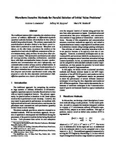
where ej is the jth canonical unit vector and m•j is the column vector representing the jth column of M . Both the construction and the application of M are embarrassingly parallel. The primary motivation to consider approximate inverse preconditioners is to exploit the rapid decay of the discrete Green’s function. As shown in Figure 1, only a very small number of entries in the exact inverse have large magnitude compared to most of the others that are much smaller. This means that a very sparse matrix is likely to retain the most relevant contributions to the inverse. The sparsity pattern of M can be computed adaptively during the computation of M itself (see e.g., [16]) or prescribed a priori based on some heuristics. We compute the pattern in advance using graph information from the mesh, by selecting for the jth column of the approximate inverse edge j and its qth level nearest-neighbors. 0

20

40

60

80

100

120 0

20

40

60 Density = 8.75%

80

100

120

Figure 1. Sparsity pattern of sparsified (A−1 ). In the last twenty years, fertile research efforts have led to the development of fast hierarchical methods for performing approximate


155

matrix-vector products with boundary integral operators (see e.g., [14– 19]), including reliable implementations on distributed memory computers [4, 20]. Hierarchical methods partition the mesh of the object by recursive subdivision into disjoint aggregates or boxes of small size compared to the wavelength, each roughly formed by an equal number of separate triangles. The box-wise decomposition of the object naturally leads to an a priori pattern selection strategy for the approximate inverse using geometric information, that is on the spatial distribution of the degrees of freedom. In the context of fast methods we will adopt the following criterion: the nonzero structure of the column of the preconditioner associated with a given edge in the mesh is defined by retaining all the edges within the box itself and one level of neighboring boxes. The preconditioner is constructed from a sparse approximation of the dense coefficient matrix, computed by retaining the entries associated with edges included in the given box as well as those belonging to two levels of neighbors. Thus the approximate inverse has a sparse block structure; each block is a dense matrix associated with one box. Indeed the least-squares problems corresponding to edges within the same box are identical because they are defined using the same nonzero structure and the same set of entries of A. It means that we only have to compute one QR factorization per box. In our implementation the size of the smallest boxes in the partitioning associated with the preconditioner is a user-defined parameter that can be tuned to control the number of nonzeros computed per column, that is the density of the preconditioner. According to our criterion, the larger the size of the boxes, the larger the geometric neighborhood that determines the sparsity structure of the columns of the preconditioner. Parallelism can be exploited by assigning disjoint subsets of boxes to different processors and performing the least-squares solutions independently on each processor. We refer to [21] for more algorithmic and implementation details of the sparse approximate inverse. To study the numerical behavior of the preconditioning algorithms described in this paper, we consider a set of test examples representative of calculations in electromagnetics applications. The tests examples are defined by: Example 1: a sphere of radius, a matrix of order n = 1080, see Figure 2(a); Example 2: a cylinder with a break on the surface, a matrix of order n = 1299, see Figure 2(b); Example 3: a Cetaf, typical test case in the electromagnetic community representing the wing of an aircraft, a matrix of order n = 86256, Figure 2(c);

156

Carpentieri

Example 4: an Airbus aircraft, a matrix of order n = 94704, Figure 2(d);

(a) Example 1

(c) Example 3

(b) Example 2

(d) Example 4

Figure 2. Mesh associated with test examples. We mention that, for physical consistency, we have set the frequency of the incident wave so that there are about ten discretization points per wavelength [22]. In Table 1 we report on comparative results with different preconditioners to compute the approximate solution on the cylinder problem. This problem can be considered representative of the general observed trend. In connection with GMRES, we consider different standard preconditioners computed from a sparse approximation A˜ of the dense coefficient matrix, all having roughly the same number of nonzero entries. In the table, we use the following acronyms:


157

• N one, means that no preconditioner is used; • Diag, the point-wise Jacobi preconditioner, i.e., a simple diagonal scaling; • SSOR, the symmetric successive overrelaxation method; • ILU (0) [23], the incomplete LU factorization with zero level of ˜ fill-in, i.e., taking for the factors the same sparsity pattern as A; • SP AI [24], a sparse approximate inverse based on Frobenius-norm minimization, with a static pattern selection strategy; • AIN V [25], a factorized approximate inverse preconditioner with a dropping strategy based on value. Table 1. Number of iterations using preconditioned GMRES on a test problem, a cylinder with an open surface, discretized with n = 1299 edges. The tolerance is set to 10−8 . The results are for right preconditioning.

Density of A˜ = 3.18% - Density of M = 1.99%. Precond. N one Diag SSOR ILU (0) SP AI AIN V

GMRES(30) +1000 +1000 +1000 +1000 308 +1000

GMRES(80) +1000 +1000 717 454 70 +1000

GMRES(∞) 302 272 184 135 70 +1000

From the numerical results reported in Table 1, we can observe that approximate inverse methods are amongst the most effective standard preconditioners on this problem class. On indefinite systems they are less prone to instabilities than incomplete factorizations that tend to compute very ill-conditioned factors and produce unstable triangular solves in GMRES. In Table 2 we show results of experiments on the numerical scalability of the sparse approximate inverse on a set of test problems arising from realistic radar cross section (RCS) calculations in industry. Large problem size is obtained by increasing the value of the frequency of the illuminating wave on the same obstacle. In these

158

Carpentieri

Table 2. Number of matrix-vector products and elapsed time required to converge on the four problems on 8 processors of the Compaq machine, except those marked with (k) , that were run on k processors. Tolerance for the iterative solution was 10−3 . Acronyms: N.A. ≡ not available. M.L.E. ≡ memory limits exceeded. Cetaf GMRES(∞)

GMRES(120)

Size

Density SPAI

Time SPAI

Iter / Time

Iter / Time

86256

0.18

4m

656 / 1h 25m

1546 / 1h 44m

134775

0.11

6m

618 / 1h 45m

1125 / 1h 55m

264156

0.06

13m

710 / 9h

1373 / 4h 46m

531900

0.03

20m

844 / 1d 18m

1717 / 14h 8m

1056636

0.01

37m

+750 / +9h(32)

+2000 / > 1d

Aircraft Size

Density SPAI

Time SPAI

GMRES(∞)

GMRES(120)

Iter / Time

Iter / Time

94704

0.28

11m

746 / 2h 9m

1956 / 3h 13m

213084

0.13

31m

973 / 7h 19m

+2000 / 7h 56m

591900

0.09

1h 30m

1461 / 16h 42m(64)

+2000 / 1d 57m

1160124

0.02

3h 24m

M.L.E.(64) / N.A.

+2000 / > 4d

experiments we use the multilevel fast multipole algorithm (MLFMA) [17] for performing approximate matrix-vector products. In the last few years active research eorts have been devoted to develop robust MLFMA techniques for solving high-frequency electromagnetic scattering problems, including efficient implementations on parallel computers (see e.g., [26–30]). Details of the implementation of our multipole code are described in [11, 32]. In Table 2 we report on the number of matrix-vector products using GMRES(30) with a required accuracy of 10−3 on the normwise backward error ||r|| ||b|| , where r denotes the residual and b the right-hand side of the linear system. We remark that this level of accuracy is in the same order of magnitude as the relative error of the matrix-vector product operation in our multipole code, estimated comparing with the level 2 BLAS routine GEMV on a small setup. This tolerance is accurate for engineering purposes, as it enables the correct construction of the radar cross section of the object.


159

All the runs have been performed in single precision on eight processors of a Compaq Alpha server. The Compaq Alpha server is a cluster of Symmetric Multi-Processors. Each node consists of four DEC Alpha processors (EV 6, 1.3 GFlops peak) that share 512 MB of memory. On that computer, the temporary disk space that can be used by the outof-core solver is around 189 GB. Among all the possible right-hand sides for each geometry, we have selected those that are the most difficult to solve in order to better illustrate the robustness and the efficiency of our preconditioner. The initial guess is the zero vector. In Table 2 “d” means day, “h” hour and “m” minute. We see that the numerical behavior of the preconditioner does not scale well with the problem size, especially GMRES(120) on the Cetaf, and there is no convergence on the largest aircraft problems. For GMRES(∞) the increase in the iteration count is less significant, even though on the Cetaf and the aircraft convergence cannot be obtained because we either exceed the memory limits of our computer or the time limit allocated to a single run. From a timing point of view, we see that the solution time of full GMRES is strongly affected by the orthogonalisation involved in the Arnoldi procedure. On the Cetaf problem discretized with 531900 points, the number of iterations of GMRES(120) is twice as large with respect to full GMRES, but GMRES(120) is about twice as cheap. Provided we get convergence, the use of a large restart often reduces the solution time even though it significantly deteriorates the convergence. On the Cetaf geometry, the solution time for the GMRES method increases superlinearly for small and medium problems, but nearly quadratically for large problems. On the largest test case, discretized with one million unknowns, unrestarted GMRES does not converge after 750 iterations requiring more than nine hours of computation on 32 processors. The Airbus aircraft is very difficult to solve because the mesh has many surface details and the discretization matrices become ill-conditioned. On small and medium problems, the number of GMRES iterations increases with the problem size, and the solution time increases superlinearly. On the largest test case, discretized with one million unknowns, full GMRES exceeds the memory limit on 64 processors. In this case, the use of large restarts (120 in this table) does not enable convergence within 2000 iterations except on a small mesh of size 94704. We see in Table 2 that our strategy for adjusting the box dimension for increasing frequencies causes the density of the sparse approximate inverse to decrease for increasing problem size. The number of unknowns per box remains constant, but the number of boxes increases leading to a decrease in density and to poorer preconditioners. Finally, in Table 3, we show the parallel scalability of the implementation of the preconditioner in the multipole code. We

160

Carpentieri

solve problems of increasing size on a larger number of processors, keeping the number of unknowns per processor constant. It can be observed the very good parallel scalability of the construction and of the application of the preconditioner; for the matrix-vector product operation, the nlogn factor appears in the results. Table 3. Parallel scalability of the code on the aircraft problem. Parallel scalability results Problem size

Nb procs

Construction

Elapsed time

Elapsed time

time (sec)

precond (sec)

mat-vec (sec)

112908

8

513

0.39

1.77

221952

16

497

0.43

2.15

342732

24

523

0.47

3.10

451632

32

509

0.48

2.80

900912

64

514

0.60

3.80

Remark. As mentioned already, our main focus is on linear systems arising from EFIE. The advantages of this formulation are numerous; in particular, it does not require any hypothesis on the geometry of the objects. We should nevertheless mention that for closed geometries the CFIE can also be used. The linear systems arising from the CFIE formulation are much easier to solve. For instance the solution of the problem associated with the aircraft with 213084 degrees of freedom requires only 129 iterations of unpreconditioned full GMRES, and 22 iterations of preconditioned full GMRES. Furthermore, preconditioned full GMRES converges in 24 iterations on the aircraft with more than a million degrees of freedom. Because the linear systems arising from the CFIE are not challenging from a linear algebra point of view, we do not consider them further in this paper. 3. SPECTRAL DEFLATION The Frobenius-norm minimization preconditioner succeeds in clustering most of the eigenvalues far from the origin. This can be observed in Figure 3 where we see a big cluster near one in the spectrum of the preconditioned matrix for a model problem that is representative of the general trend. However, it tends to leave a few very small eigenvalues close to the origin that can slow down the convergence significantly (see [31]).


161

0.5

Imaginary axis

0

0.5

1

1.5

0.5

0

0.5 Real axis

1

1.5

Figure 3. Eigenvalue distribution for the coefficient matrix preconditioned by the Frobenius-norm minimization method on a model problem that is representative of the general trend. In this section, we propose a refinement technique which enhances the robustness of the approximate inverse by removing the effect of the smallest eigenvalues in magnitude in the preconditioned matrix. The proposed technique is based on the introduction of low-rank corrections computed by using spectral information associated with the smallest eigenvalues in M A. Roughly speaking, we solve the preconditioned system exactly on a coarse space and use this information to update the preconditioned residual. We consider the linear system Ax = b,

(3)

where A is a n×n complex unsymmetrical nonsingular matrix, x and b are vectors of size n. The linear system is solved using a preconditioned Krylov solver and we denote by M1 the left preconditioner, meaning that we solve M1 Ax = M1 b.

(4)

We assume that the preconditioned matrix M1 A is diagonalizable,

162

Carpentieri

that is: M1 A = V ΛV −1 ,

(5)

with Λ = diag(λi ), where |λ1 | ≤ . . . ≤ |λn | are the eigenvalues and V = (vi ) the associated right eigenvectors. We denote by U = (ui ) the associated left eigenvectors; we then have U H V = diag(uH i vi ), with uH v = 0, ∀i [32]. Let V be the set of right eigenvectors associated ε i i with the set of eigenvalues λi with |λi | ≤ ε. Similarly, we define by Uε the corresponding subset of left eigenvectors. The following results are simple to derive. Theorem 1 Let Ac = UεH M1 AVε , H Mc = Vε A−1 c Uε M1

and M = M1 + Mc . Then M A is diagonalisable and we have M A = V diag(ηi )V −1 with ηi = λi if |λi | > ε, ηi = 1 + λi if |λi | ≤ ε. Ac represents the projection of the matrix M1 A on the coarse space defined by the approximate eigenvectors associated with its smallest eigenvalues. Theorem 2 Let W be such that A˜c = W H AVε has full rank, H ˜ c = Vε A˜−1 M c W and

˜ c. ˜ = M1 + M M

˜ A is similar to a matrix whose eigenvalues are Then M ηi = λi if |λi | > ε, ηi = 1 + λi if |λi | ≤ ε. For right preconditioning, that is AM1 y = b, similar results hold. Lemma 1 Let Ac = UεH AM1 Vε , H Mc = M1 Vε A−1 c Uε


163

and M = M1 + Mc . Then AM is diagonalisable and we have AM = V diag(ηi )V −1 with ηi = λi if |λi | > ε, ηi = 1 + λi if |λi | ≤ ε. Lemma 2 Let W be such that A˜c = W H AM1 Vε has full rank, H ˜ c = M1 Vε A˜−1 M c W and

˜ c. ˜ = M1 + M M

˜ is similar to a matrix whose eigenvalues are Then AM if |λi | > ε, ηi = λi ηi = 1 + λi if |λi | ≤ ε. We should point out that in the nonsymmetric case a natural choice exists for the operator W , i.e., to select W = Vε , that saves the computation of left eigenvectors. We also mention that an additional scaling can be introduced in the low-rank update so that the k smallest eigenvalues are not just shifted by one, but rather are all transformed to one with multiplicity equal to k. This feature can H be obtained by using Mc = Vε (I − Dε )A−1 c Uε in Proposition 1, and −1 H Mc = Vε (I − Dε )Ac W in Proposition 2. Similar transformations can be applied to get the same property for right preconditioning. We report on experiments to illustrate the effectiveness of the spectral preconditioning updates when used to accelerate restarted GMRES. For ease of presentation, we compute the eigenpairs in a preprocessing step, that is before solving the linear system. We mention that the standard implementation of the GMRES algorithm is based on the Arnoldi process, and this allows us to recover spectral information of A during the iterations [33]. We use the IRA method implemented in the ARPACK package [34] to compute approximations to the smallest eigenvalues and their corresponding approximate eigenvectors. This makes the preconditioner independent of the Krylov solver. We consider the formulation described in Proposition 2 that requires computation of only right eigenvectors and we apply the spectral updates on top of the preconditioned system AM1 x = b. The first level preconditioner M1 is the Frobenius-norm minimization method introduced earlier. All the numerical experiments are performed in

164

Carpentieri

Table 4. Number of iterations required by GMRES preconditioned by a Frobenius-norm minimization method updated with spectral corrections to reduce the normwise backward error by 10−8 for increasing size of the coarse space. Cylinder problem Size of the coarse space 0 4 8 12 16 20

GMRES(m), Toler. 1e-8 m=10 +500 279 188 196 183 168

m=30 +500 192 147 148 137 130

m=50 496 152 129 131 114 100

m=80 311 125 90 91 74 69

m=110 198 93 84 83 74 69

Sphere problem Size of the coarse space 0 4 8 12 16 20

GMRES(m), Toler. 1e-8 m=10 297 345 55 52 52 53

m=30 87 66 43 43 44 45

m=50 75 64 40 38 39 40

m=80 66 58 40 38 39 40

m=110 66 58 40 38 39 40

double precision complex arithmetic on a SGI Origin 2000 and the number of iterations are for right preconditioning. In Table 4 we show the number of iterations required by GMRES to obtain convergence for increasing size of the coarse space up to twenty on the cylinder problem and on the sphere. In these experiments, the small problem size enables us to carry out the matrix-vector products exactly, i.e., using the level 2 BLAS routine GEMV. Thus the tolerance adopted in the stopping criterion for GMRES, that is related to the normwise


165

Table 5. Effect of shifting the eigenvalues nearest zero on the convergence of GMRES(30). We show the magnitude of successively shifted eigenvalues and the number of iterations required when these eigenvalues are shifted. Cylinder problem Nr of shifted

Magnitude of

GMRES(30)

Eigenvalues

the eigenvalue

Toler = 10−8

0

+1500

1

7.1116e-04

215

2

4.9685e-02

202

3

5.2737e-02

193

4

6.3989e-02

192

5

7.0395e-02

190

6

7.7396e-02

189

7

7.8442e-02

161

8

8.9548e-02

147

9

9.1598e-02

146

10

9.9216e-02

144

Sphere problem Nr of shifted

Magnitude of

GMRES(30)

Eigenvalues

the eigenvalue

Toler = 10−8

0

87

1

8.7837e-03

79

2

8.7968e-03

79

3

8.7993e-03

66

4

9.8873e-03

66

5

9.9015e-03

66

6

9.9053e-03

66

7

9.9126e-03

43

8

2.3331e-01

43

9

2.4811e-01

43

10

2.4813e-01

44

166

Carpentieri

backward error, is significantly smaller than in the runs with MLFMA reported in the previous section. We can see that the introduction of the low-rank updates can remarkably accelerate the iterative solution. By selecting up to ten eigenpairs the number of iterations decreases by at least a factor of two. On the cylinder problem the preconditioning updates enable fast convergence of GMRES with a low restart whereas no convergence was obtained in 1500 iterations without updates. The remarkable robustness of the preconditioner enables the use of very small restarts for GMRES. We observe that the gain in terms of iterations is strongly related to the magnitude of the shifted eigenvalues. A speedup in convergence is obtained when a full cluster of small eigenvalues is completely removed from the spectrum. This is illustrated in Tables 5 where we show the effect of deflating eigenvalues of increasing magnitude on the convergence of GMRES(30). On the cylinder, the presence of one very small eigenvalue slows down the convergence significantly. Once this eigenvalue is shifted, the number of iterations rapidly decreases. On the sphere, there is a cluster of seven eigenvalues of magnitude around 10−3 . When the eigenvalues within the cluster are shifted, a quick speedup of convergence is observed; the shifting of the remaining eigenvalues does not have any impact on the convergence. The application of the correction update at each iteration step costs 2nk + k 2 , where k is the size of the coarse space. The setup of the preconditioner is more expensive. In Table 6 we show the number of matrix-vector products required by the ARPACK implementation of the IRA method to compute the smallest approximate eigenvalues and the associated approximate right eigenvectors. The matrix-vector products do not include those required for the iterative solution. We see that the computation can be fairly expensive but the cost can be amortized if the preconditioner is reused to solve linear systems with the same coefficient matrix and several right-hand sides. This is the typical scenario in realistic electromagnetic simulations. In bistatic radar cross section calculations, linear systems with the same coefficient matrix and up to hundreds of different right-hand sides are solved, ranging over the complete set of directions between the transmitter and the receiver. In Table 6 we also show the number of amortization vectors relative to GMRES(10), that is the number of right-hand sides that have to be considered to amortize the extra cost for the eigencomputation. A multilevel algorithm based on spectral deflation is introduced in [35]; the idea is inherited from standard two-grid cycles that are fully defined by the selection of the coarse grid, the choice of the smoother applied on the fine grid and of the grid transfer operators to move


167

Table 6. Number of matrix-vector products required by the IRA algorithm to compute approximate eigenvalues nearest zero and the corresponding right eigenvectors. Cost of spectral deflation Size of the coarse space 4 8 12 16 20

M-V products Cylinder 469 333 579 1053 1066

Sphere 103 105 131 237 220

Amortization Cylinder 1 1 1 1 1

Sphere 1 1 1 1

between fine and coarse grid. In [35], the preconditioner M is used to define a weighted stationary method that implements the smoother and the coarse space is defined using a Galerkin formula Ac = RH AP , where R and P are the restriction and the prolongation operator, respectively. After µ smoothing steps, the residual is projected into the coarse subspace by means of the operator R and the coarse space error equation involving Ac = RH AP is solved exactly. Finally, the error is prolongated back in the original space using the operator P and the new approximation is smoothed again. These two contributions are summed together for the solution update. We define the gridtransfer operators algebraically, and select P = Vε to be the set of right eigenvectors associated with the set of eigenvalues λi of M1 A with |λi | ≤ ε. For the restriction operator, a natural choice is to select R = W orthogonal to Vε (i.e., W H Vε = I). Following [36, 37], we define the filtering operators using the grid transfer operators as (I − Vε W H ). Thus we have (I − Vε W H )Vε = 0 and the filtering operator is supposed to remove all the components of the preconditioned residual in the Vε directions. The coarse grid correction computes components of the residual in the space spanned by the eigenvectors associated with the few selected small eigenvalues, while at the end of the smoothing step the preconditioned residual is filtered so that only components in the complementary subspace are retained. The preconditioner constructed using this scheme depends on A, M1 , µ, ω > 0. For the sake of simplicity of exposure, we will simply denote it by MAdd (A, M1 ). A

168

Carpentieri

sketch of the algorithm is presented in Figure 4. It takes as input a vector r that is the residual vector we want to precondition, and returns as output the preconditioned residual vector z.

Figure 4. Additive two-grid spectral preconditioning. The algorithm. Proposition 1 Let W be such that Ac = W H AVε has full rank and satisfies (I − Vε W H )Vε = 0, the preconditioning operation described in the algorithm of Figure 4 can be written in the form z = MAdd r. After one cycle (iter = 1), MAdd has the following expression: H + (I − Vε W H )(I − (I − ωM1 )µ )A−1 . MAdd = Vε A−1 c W

(6)

In the following proposition we examine the effect of MAdd on the spectrum of the preconditioned matrix. As before, we assume that M1 A has a standard eigendecomposition M1 A = V ΛV −1 ,

(7)


169

with Λ = diag(λi ), where |λ1 | ≤ . . . ≤ |λn | are the eigenvalues and V = (vi ) the associated right eigenvectors. We denote Vε be the set of right eigenvectors associated with the set of eigenvalues λi with |λi | ≤ ε. Proposition 2 The preconditioner MAdd defined by Proposition 1 is such that the preconditioned matrix MAdd A has eigenvalues: ηi = 1 if |λi | ≤ ε, ηi = 1 − (1 − ωλi )µ if |λi | > ε. The effect of the coarse grid correction that shifts the smallest eigenvalues to one combined with a few Richardson iterations that cluster the rest of the spectrum can be beneficial in the presence of outliers or many isolated eigenvalues. The price to pay are additional matrix-vector products. Applying MAdd requires (µ − 1) × iter matrixvector products with M1 , and (µ×iter−1) products by A. The filtering operation costs 2nk operations and the low frequency correction costs 2nk + k 2 , where k is the size of the coarse space. As µ, iter, k are O(1), the overall cost of applying MAdd if O(n). In Table 7 we show results of experiments on the Airbus aircraft problem discretized with 23796 nodes. We have seen that, although small, this problem is difficult to solve by iterative methods. Using GMRES and the Frobenius-norm minimization preconditioner, convergence is achieved only with large values of restart. It can be observed that the use of MAdd is very beneficial. Using only ten eigenvectors, the preconditioner enables to obtain convergence for very small restart (i.e., low memory complexity). We note that the larger the coarse space, the better the preconditioner; both the number of GMRES iterations and the solution time decrease when the number of smoothing steps is increased. Experiments on a larger set of problems are found in [35, 38]. Table 7. Experiments with MAdd on the Airbus aircraft problem. Airbus aircraft problem (size 94704) With MSP AI GMRES(10) +4000 iterations µ GMRES(10) CPU-time 1 1835 1h 07m 2 807 36m 3 368 22m

170

Carpentieri

Figure 5. Inner-outer solution schemes in the multipole context. Sketch of the algorithm. 4. INNER-OUTER ITERATIVE SCHEMES In this section we report on experiments with inner-outer solution schemes implemented in the multipole context, with the intent of recovering global information of the discrete Green’s function fort solving large problems. The motivation that naturally leads us to consider inner-outer schemes is to try to balance the locality of the preconditioner with the use of the multipole matrix. The underlying idea is simply to carry out a few steps of an inner Krylov method for the preconditioning operation. The overall algorithm is sketched in Figure 5. The outer solver must be able to work with variable preconditioners. Amongst various possibilities, we mention FGMRES [39] and GMRES6 [40, p. 91]; this latter reduces to GMRESR [41] when the inner solver is GMRES. The efficiency of the proposed algorithm relies on two main factors: the inner solver has to be preconditioned so that the residual in the inner iterations can be significantly reduced in a few steps, and the matrix-vector products within the inner and the outer solvers can be carried out with a different accuracy. Experiments conducted in [42] with inner-outer schemes combined with multipole techniques on the potential equation were not entirely successful. In that case, no preconditioner was used in the inner solver. The desirable feature of using different accuracies for the matrix-vector products is enabled by the use of the MLFMA. In our


171

scheme, a highly accurate MLFMA is used within the outer solver as it governs the final accuracy of the computed solution. A less accurate MLFMA is used within the inner solver as it is a preconditioner for the outer scheme; in this respect the inner iterations only attempt to give a rough approximation of the solution and consequently do not require an accurate matrix-vector calculation. In fact, we solve a nearby system for the preconditioning operation, that enables us to save considerable computational effort during the iterative process as the less accurate matrix-vector calculation requires about half of the computing time of the accurate one. In Table 8, we show the average elapsed time in seconds observed on eight processors for a matrix-vector product using the MLFMA with different accuracy levels. Table 8. Average elapsed time observed on eight processors in seconds for a matrix-vector product using the MLFMA with different levels of accuracy. Cost of MLFMA Geometry inner MLFMA outer MLFMA Airbus 94704 3.5 4.8 Airbus 213084 6.9 11.8 Airbus 591900 17.4 30.2 Airbus 1160124 34.5 66.5 In the experiments reported in this section, we consider FGMRES as the outer solver with an inner GMRES iteration preconditioned with the Frobenius-norm minimization method. For the FGMRES method, we consider the implementation described in [43]. The convergence history of GMRES depicted in Figure 6 for different values of the restart gives us some clues to the numerical behavior of the proposed scheme. The residual of GMRES tends to decrease very rapidly in the first few iterations independently of the restarts, then decreases much more slowly, and finally stagnates to a value that depends on the restart; the larger the restart, the lower the stagnation value. It suggests that a few steps in the inner solver can be very effective for obtaining a significant reduction of the initial residual. In Table 9, we describe the results of experiments on an Airbus aircraft with 213084 points using different combinations of restarts for the inner and outer solvers. If the number of inner steps is too small, the preconditioning operation is poor and the convergence slows down, while too large restarts of GMRES tend to increase the overall computational cost

172

Carpentieri 10

Log10 (normwise backward error)

restart = 10 restart = 60 restart = 500

1

10

2

10

3

10

0

100

200

300

400 500 600 Number of iterations

700

800

900

1000

Figure 6. Convergence history of restarted GMRES for different values of restart on the aircraft problem discretized with 94704 points. but do not cause further reduction of the normwise backward error at the beginning of convergence. The choice of the restart for the outer solver depends to a large extent on the available memory of the target machine and the difficulty of the problem at hand, an issue that is also related to the illuminating direction of the incident wave that defines the right-hand side. Amongst the various possibilities, we select FGMRES(30) and GMRES(60) on the Airbus aircraft and the Cetaf problem. These combinations are a good trade-off. In Table 10 we show the results of experiments on the same geometries that we considered in Section 2. We show the number of inner and outer matrix-vector products and the elapsed time needed to achieve convergence using a tolerance of 10−3 on eight processors of the Compaq machine. In the runs, we use MLFMA for the matrix-vector products. It can be seen that the combination FGMRES/GMRES remarkably enhances the robustness of the preconditioner especially on large problems. The increase in the number of outer iterations is fairly modest except on the largest aircraft test cases. Nevertheless, the scheme is the only one that enables us to get the solution of this challenging problem since classical restarted GMRES does not converge and full GMRES exceeds the memory of our computer. Similarly,


173

Table 9. Global elapsed time and total number of matrix-vector products required to converge on an Airbus aircraft with 213084 points varying the inner restart parameter. The runs have been performed on 8 processors of the Compaq machine. restart

restart

# total inner

# total outer

FGMRES

GMRES

mat-vec

mat-vec

30

40

1960

51

4h 58m

30

50

1900

40

4h 53m

30

60

1920

34

4h 55m

30

70

2030

30

5h 13m

30

80

2240

29

5h 50m

times

Table 10. Number of matrix-vector products and elapsed time required to converge on 8 processors of the Compaq machine. The tests were run on 8 processors of the Compaq machine, except those marked with (k) , that were run on k processors. Cetaf Size

Density SPAI

Time SPAI

FGMRES(30)/GMRES(60) Iter

Time

4m

17+ 960

55m

86256

0.18

134775

0.11

6m

15+ 840

1h 19m

264156

0.06

13m

17+ 960

2h 22m

531900

0.03

20m

19+1080

6h

1056636

0.01

37m

22+1260

14h

Aircraft Size

FGMRES(30)/GMRES(60)

Density SPAI

Time SPAI

Iter

Time

94704

0.28

11m

27+1560

2h 14m

213084

0.13

31m

34+1920

5h

591900

0.09

1h 30m

57+3300

1d 9h 45m

1160124

0.02

3h 24m

51+2940

16h 41m(64)

174

Carpentieri

on the Cetaf discretized with one million points, the embedded scheme enables us to get convergence in 22 outer iterations, whereas GMRES(120) does not converge in 2000 iterations. The saving in time is also noticeable. The gain ranges from two to four depending on the geometry and tends to become larger when the problem size increases. 5. CONCLUSIONS In this paper we have described an effective and inherently parallel approximate inverse preconditioner based on a Frobenius-norm minimization preconditioner, that can easily be implemented in a fast multipole code. We have studied the numerical scalability of our method for the solution of very large dense linear systems of equations arising in realistic electromagnetic scattering simulations. We have described multilevel strategies based on spectral preconditioning that induce a global deflation of the eigenvalues of the preconditioned matrix. The transformation can result in a well clustered spectrum around one that is more amenable to iterative solvers. The experiments show that the proposed scheme is fairly robust, requires limited memory, is easy to combine with multipole techniques and is matrixfree as it does not require the explicit computation of all the entries of the coefficient of the linear system to solve. We have illustrated how to improve the locality of the sparse approximate inverse on large problems by embedding the preconditioner within inner-outer solution schemes based on the GMRES method, implemented in a multipole context using different levels of accuracy for the matrix-vector products. We have shown that the combination FGMRES/GMRES can effectively enhance the robustness of the preconditioner and reduce significantly the computational cost and the storage requirements for the solution of large problems. Most of the experiments reported in this paper require a huge amount of computation and storage, and they often reach the limits of our target machine in terms of memory and disk storage. To give an idea of how large these simulations are, the solution of systems with one million unknowns using a direct method would require 8 Tbytes of storage and 37 years of computation on one processor of the target computer (assuming the computation runs at peak performance). Such simulations are nowadays feasible thanks to the use of iterative methods and can be integrated in the design processes where the bottleneck moves from the simulation to the pre and post-processing of the results as the tools are not yet available to easily manipulate meshes with millions of degrees of freedom.


175

ACKNOWLEDGMENT This research was possible thanks to the computing facilities and to the fertile working environment of the CERFACS institute (Toulouse, France). Part of the work was supported by I.N.D.A.M. (Rome, Italy) under a grant (Borsa di Studio per l’estero, Provvedimento del Presidente del 30 Aprile 1998). The author would like to thank Guillaume Alléon from EADS-CCR (European Aeronautic Defence and Space - Company Corporate Research Center) located in Toulouse, for providing us some test examples considered in this paper, and Guillaume Sylvand from EADS-CCR for providing with the multipole code and valuable support. REFERENCES 1. Jin, K. S., T. I. Suh, S. H. Suk, B. C. Kim, and H. T. Kim, “Fast ray tracing using a space-division algorithm for rcs prediction,” Journal of Electromagnetic Waves and Applications, Vol. 20, No. 1, 119–126, 2006. 2. Wang, Y. B., Y. M. Bo, and D. Ben, “Fast rcs computation with general asymptotic waveform evaluation,” Journal of Electromagnetic Waves and Applications, Vol. 12, 1873–1884, 2007. 3. Wang, S., X. Guan, D. Wang, X. Ma, and Y. Su, “Fast calculation of wide-band responses of complex radar targets,” Progress In Electromagnetics Research, PIER 68, 185–196, 2007. 4. Sylvand, G., “La méthode multipˆ ole rapide en electromagnétisme: Performances, parallélisation, applications,” Ph.D. thesis, Ecole Nationale des Ponts et Chaussées, 2002. 5. Rao, S. M., D. R. Wilton, and A. W. Glisson, “Electromagnetic scattering by surfaces of arbitrary shape,” IEEE Trans. Antennas Propagat., Vol. AP-30, 409–418, 1982. 6. Chew, W. C. and K. F. Warnick, “On the spectrum of the electric field integral equation and the convergence of the moment method,” Int. J. Numerical Methods in Engineering, Vol. 51, 475– 489, 2001. 7. Song, J., C.-C. Lu, and W. C. Chew, “Multilevel fast multipole algorithm for electromagnetic scattering by large complex objects,” IEEE Transactions on Antennas and Propagation, Vol. 45, No. 10, 1488–1493, 1997. 8. Sertel, K. and J. L. Volakis, “Incomplete LU preconditioner for

176

9.

10.

11.

12.

13.

14. 15.

16.

17.

18. 19.

20. 21.

Carpentieri

FMM implementation,” Micro. Opt. Tech. Lett., Vol. 26, No. 7, 265–267, 2000. Lee, J., C.-C. Lu, and J. Zhang, “Incomplete LU preconditioning for large scale dense complex linear systems from electromagnetic wave scattering problems,” J. Comp. Phys., Vol. 185, 158–175, 2003. Carpentieri, B., I. S. Duff, L. Giraud, and M. Magolu monga Made, “Sparse symmetric preconditioners for dense linear systems in electromagnetism,” Numerical Linear Algebra with Applications, Vol. 11, No. 8–9, 753–771, 2004. Ewe, W.-B., L.-W. Li, Q. Wu, and M.-S. Leong, “Preconditioners for adaptive integral methods implementation,” IEEE Transactions on Antennas and Propagation, Vol. 53, No. 7, 2346–2350, 2005. Malas, T. and L. G¨ urel, “Incomplete LU preconditioning with multilevel fast multipole algorithm for electromagnetic scattering,” SIAM J. Scientific Computing, Vol. 29, No. 4, 1476– 1494, 2007. Gould, N. I. M. and J. A. Scott, “Sparse approximate-inverse preconditioners using norm-minimization techniques,” SIAM J. Scientific Computing, Vol. 19, No. 2, 605–625, 1998. Bebendorf, M., “Approximation of boundary element matrices,” Numerische Mathematik, Vol. 86, No. 4, 565–589, 2000. Bebendorf, M. and S. Rjasanov, “Adaptive low-rank approximation of collocation matrices,” Computing, Vol. 70, No. 1, 1–24, 2003. Canning, F. X., “The impedance matrix localization (IML) method for moment-method calculations,” IEEE Antennas and Propagation Magazine, 1990. Greengard, L. and V. Rokhlin, “A fast algorithm for particle simulations,” Journal of Computational Physics, Vol. 73, 325–348, 1987. Hackbush, W., “A sparse matrix arithmetic based on H-matrices,” Computing, Vol. 62, No. 2, 89–108, 1999. Hackbush, W. and Z. P. Nowak, “On the fast matrix multiplication in the boundary element method by panel clustering,” Numerische Mathematik, Vol. 54, No. 4, 463–491, 1989. Greengard, L. and W. Gropp, “A parallel version of the fast multipole method,” Comput. Math. Appl., Vol. 20, 63–71, 1990. Carpentieri, B., I. S. Duff, L. Giraud, and G. Sylvand,


22.

23. 24.

25.

26.

27.

28. 29.

30.

31.

32. 33. 34.

177

“Combining fast multipole techniques and an approximate inverse preconditioner for large electromagnetism calculations,” SIAM J. Scientific Computing, Vol. 27, No. 3, 774–792, 2005. Bendali, A., “Approximation par elements finis de surface de problemes de diffraction des ondes electro-magnetiques,” Ph.D. thesis, Université Paris VI, 1984. Saad, Y., Iterative Methods for Sparse Linear Systems, PWS Publishing, New York, 1996. Grote, M. and T. Huckle, “Parallel preconditionings with sparse approximate inverses,” SIAM J. Scientific Computing, Vol. 18, 838–853, 1997. Benzi, M., C. D. Meyer, and M. Touma, “A sparse approximate inverse preconditioner for the conjugate gradient method,” SIAM J. Scientific Computing, Vol. 17, 1135–1149, 1996. Wang, P., Y. J. Xie, and R. Yang, “Novel pre-corrected multilevel fast multipole algorithm for electrical large radition problem,” Journal of Electromagnetic Waves and Applications, Vol. 11, 1733–1743, 2007. Pan, X. M. and X. Q. Sheng, “A highly efficient parallel approach of multi-level fast multipole algorithm,” Journal of Electromagnetic Waves and Applications, Vol. 20, No. 8, 1081– 1092, 2006. Darve, E., “The fast multipole method: Numerical implementation,” J. Comp. Phys., Vol. 160, No. 1, 195–240, 2000. Zhao, X. W., X.-J. Dang, Y. Zhang, and C.-H. Liang, “The multilevel fast multipole algorithm for emc analysis of multiple antennas on electrically large platforms,” Progress In Electromagnetics Research, PIER 69, 161–176, 2007. Zhang, Y. J. and E. P. Li, “Fast multipole accelerated scattering matrix method for multiple scattering of a large number of cylinders,” Progress In Electromagnetics Research, PIER 72, 105– 126, 2007. Greenbaum, A., Iterative Methods for Solving Linear Systems, Frontiers in Applied Mathematics, No. 17, SIAM, Philadelphia, 1997. Wilkinson, J. H., The Algebraic Eigenvalue Problem, Oxford University Press, Walton Street, Oxford OX2 6DP, UK, 1965. Trefethen, L. N. and III D. Bau, Numerical Linear Algebra, SIAM Book, Philadelphia, 1997. Lehoucq, R., D. Sorensen, and P. Vu, ARPACK User’s Guide: Solution of LargeScale Eigenvalue Problems with Implicitly

178

35.

36.

37.

38.

39.

40. 41.

42.

43.

Carpentieri

Restarted Arnoldi Methods, Society for Industrial and Applied Mathematics, Philadelphia, 1998. Carpentieri, B., “A matrix-free two-grid preconditioner for boundary integral equations in electromagnetism,” Computing, Vol. 77, No. 3, 275–296, 2006. Fournier, L. and S. Lanteri, “Multiplicative and additive parallel multigrid algorithms for the acceleration of compressible flow computations on unstructured meshes,” Applied Numerical Mathematics, Vol. 36, 401–426, 2001. Tuminaro, R. S., “A highly parallel multigrid-like method for the solution of the Euler equations,” SIAM J. Scientific and Statistical Computing, Vol. 13, 88–100, 1992. Carpentieri, B., L. Giraud, and S. Gratton, “Additive and multiplicative two-level spectral preconditioning for general linear systems,” SIAM J. Scientific Computing, Submitted, 2006. Saad, Y., “A flexible inner-outer preconditioned GMRES algorithm,” SIAM J. Scientific and Statistical Computing, Vol. 14, 461–469, 1993. Van der Vorst, H. A., Iterative Krylov Methods for Large Linear Systems, Cambridge University Press, Cambridge, UK, 2003. Van der Vorst, H. A. and C. Vuik, “GMRESR: A family of nested GMRES methods,” Numerical Linear Algebra with Applications, Vol. 1, 369–386, 1994. Grama, A., V. Kumar, and A. Sameh, “Parallel hierarchical solvers and preconditioners for boundary element methods,” SIAM J. Scientific Computing, Vol. 20, No. 1, 337–358, 1999. Frayssé, V., L. Giraud, S. Gratton, and J. Langou, “A set of GMRES routines for real and complex arithmetics on high performance computers,” Technical Report TR/PA/03/3, CERFACS, Toulouse, France, 2003.