(Right) Our frequency-domain modal synthesis exploits the inherent sparsity of the modes' discrete. Fourier transforms to obtain lower costs per frame. ence.
Fast Modal Sounds with Scalable Frequency-Domain Synthesis Nicolas Bonneel∗ George Drettakis∗ Nicolas Tsingos Isabelle Viaud-Delmon REVES/INRIA Sophia-Antipolis CNRS-UPMC UMR 7593
Doug James Cornell University
Abstract
1
Introduction
The rich content of today’s interactive simulators and video games includes physical simulation, typically provided by efficient physics engines, and 3D sound rendering, which greatly increases our sense of presence in the virtual world [Larsson et al. 2002]. Physical simulations are a major source of audio events: e.g., debris from explosions or impacts from collisions (Fig. 1). In recent work several methods have been proposed to physically simulate these audio events notably using modal synthesis [O’Brien et al. 2002; van den Doel and Pai 2003; James et al. 2006]. Such simulations result in a much richer virtual experience compared to simple recorded sounds due to the added variety and improved audio-visual coher∗ e-mail:
{Nicolas.Bonneel|George.Drettakis}@sophia.inria.fr
+
{
M modes
...
1024 samples 1024 samples 1024 samples
5 bins
5 bins
Amplitude
11.6 msec
{
5 bins
+
5 bins
+
5 bins
frequency
5 bins
Cost per frame ~M x 1024
5 bins
5 bins
{
{
{
+
5 bins
Cost per frame ~M x 5
iFFT (once per frame for ALL sounds)
Amplitude
Keywords: Sound synthesis, modal synthesis, real-time audio rendering, physically based animation
{
1024 samples 1024 samples 1024 samples
time
11.6 msec
{
11.6 msec
{
11.6 msec
...
11.6 msec
{
11.6 msec
1024 samples 1024 samples 1024 samples
CR Categories: I.6.8 [Simulation and Modeling]: Types of Simulation—Animation, I.3.5 [Computer Graphics]: Computational Geometry and Object Modeling—Physically based modeling I.3.7 [Computer Graphics]: Three-Dimensional Graphics and Realism—Virtual Reality
Sparse Frequency-domain Modal Synthesis
Time-domain Modal Synthesis Amplitude
Audio rendering of impact sounds, such as those caused by falling objects or explosion debris, adds realism to interactive 3D audiovisual applications, and can be convincingly achieved using modal sound synthesis. Unfortunately, mode-based computations can become prohibitively expensive when many objects, each with many modes, are impacted simultaneously. We introduce a fast sound synthesis approach, based on short-time Fourier Tranforms, that exploits the inherent sparsity of modal sounds in the frequency domain. For our test scenes, this “fast mode summation” can give speedups of 5-8 times compared to a time-domain solution, with slight degradation in quality. We discuss different reconstruction windows, affecting the quality of impact sound “attacks”. Our Fourier-domain processing method allows us to introduce a scalable, real-time, audio processing pipeline for both recorded and modal sounds, with auditory masking and sound source clustering. To avoid abrupt computation peaks, such as during the simultaneous impacts of an explosion, we use crossmodal perception results on audiovisual synchrony to effect temporal scheduling. We also conducted a pilot perceptual user evaluation of our method. Our implementation results show that we can treat complex audiovisual scenes in real time with high quality.
1024 samples 1024 samples 1024 samples
time
Output Sound
Figure 1: Frequency-domain fast mode summation: Top: Frames of some of the test scenes our method can render in real time. Bottom: (Left) Time-domain modal synthesis requires summing all modes at every sample. (Right) Our frequency-domain modal synthesis exploits the inherent sparsity of the modes’ discrete Fourier transforms to obtain lower costs per frame.
ence. The user’s audiovisual experience in interactive 3D applications is greatly enhanced when large numbers of such audio events are simulated. Previous modal sound approaches perform time-domain synthesis [van den Doel and Pai 2003]. Recent interactive methods progressively reduce computational load by reducing the number of modes in the simulation [Raghuvanshi and Lin 2006; van den Doel et al. 2004]. Their computational overload however is still too high to handle environments with large numbers of impacts, especially given the limited budget allocated to sound processing, as is typically the case in game engines. Interactive audiovisual applications also contain many recorded sounds. Recent advances in interactive 3D sound rendering use frequency-domain approaches, effecting perceptually validated progressive processing at the level of Fourier Transform coefficients [Tsingos 2005]. For faster interactive rendering, perceptually based auditory masking and sound-source clustering can be used [Tsin-
gos et al. 2004; Moeck et al. 2007]. These algorithms enable the use of high-quality effects such as Head-Related Transfer Function (HRTF) spatialization, but are limited to pre-recorded sounds. While the provision of a common perceptually based pipeline for both recorded and synthesized sounds would be beneficial, it is not directly obvious how modal synthesis can be efficiently adapted to benefit from such solutions. In the particular case of contact sounds, a frequency-domain representation of the signal must be computed on-the-fly, since events causing the sounds are triggered and controlled in real-time using the output of the physics engine.
physics engine (impact, contact etc.); we assume that this sound is synthesized on-the-fly.
Our solution to the above problems is based on a fundamental intuition: modal sounds have an inherently sparse representation in the frequency domain. We can thus perform frequency-domain modal synthesis by fast summation of a small number of Fourier coefficients (see Fig. 1). To do this, we introduce an efficient approximation to the short-time Fourier Transform (STFT) for modes. Compared to time-domain modal synthesis [van den Doel and Pai 2003], we observe 5-8 times speedup in our test scenes, with slight degradation in quality. Quality is further degraded for sounds with faster decays and high frequencies.
computed vibration modes of the objects by the contact force to synthesize the corresponding audio signal. In our context, this force is most often provided by a real-time physics engine. The acoustic response of an object to an impulse is given by:
In addition to the inherent speed-up, we can integrate modal and recorded sounds into a common pipeline, with fine-grain scalable processing as well as auditory masking and sound clustering. To compute our STFT we use a constant exponential approximation; we also reconstruct with an Hann window to simplify integration in the full pipeline. However, these approximations reduce the quality of the onset of the impact sound or “attack”. We propose a method to preserve the attacks (see Sect. 4.3), which can be directly used for modal sounds; using it in the combined pipeline is slightly more involved. We use the Hann window since it allows better reconstruction with a small number of FFT coefficients compared to a rectangular window. A rectangular window is better at preserving the attacks, but results in ringing. Our attack-preserving approach starts with a rectangular subwindow, followed by appropriate Hann subwindows for correct overlap with subsequent frames. In contrast to typical usage of pre-recorded ambient sounds, physics-driven impact sounds often create peaks of computation load, for example the numerous impacts of debris just after an explosion. We exploit results from human perception to perform temporal scheduling, thus smoothing out these computational peaks. We also performed a perceptually based user evaluation both for quality and temporal scheduling. In summary, our paper has the following contributions: • A fast frequency-domain modal synthesis algorithm, leveraging the sparsity of Fourier transforms of modal sounds. • A full, perceptually based interactive audio rendering pipeline with scalable processing, auditory masking and sound source clustering, for both recorded and modal sounds. • A temporal scheduling approach based on research in perception, which smooths out computational peaks due to the sudden occurrence of a large number of impact sounds. • A pilot perceptual user study to evaluate our algorithms and pipeline. We have implemented our complete pipeline; we present interactive rendering results in Sect. 7 and in the accompanying video for scenes such as those shown in Fig. 1 and Fig. 6.
2
Previous Work
There is extensive literature on sound synthesis and on spatialization for virtual environments. We discuss here only a small selection of methods directly related to our work: contact sound synthesis in the context of virtual environments, audio rendering of complex soundscapes, and finally crossmodal perception, which we use to smooth computational peaks. Contact sound synthesis Modal synthesis excites the pre-
s(t) = ∑ ak e−αk t sin(ωk t),
(1)
k
where s(t) is the time-domain representation of the signal, ωk is the angular frequency and αk is the decay rate of mode k; ak is the amplitude of the mode, which is calculated on the fly (see below), and may contain a radiation factor (e.g., see [James et al. 2006]). Eq. 1 can be efficiently implemented using a recursive formulation [van den Doel and Pai 2003] which makes modal synthesis attractive to represent contact sounds, both in terms of speed and memory. We define mk (t) as follows for notational convenience: mk (t) = e−αk t sin(ωk t)
(2)
The modal frequencies ωk ’s and decay rates αk ’s can be precomputed by simulating the mechanical behavior of each specific object independently. Such simulations can be done through finite elements methods [O’Brien et al. 2002], spring-mass system [Raghuvanshi and Lin 2006], or even with analytic solutions for simple cases [van den Doel et al. 2004]. The only quantities which must be computed at run-time are the gains ak since they depend on the contact position on the objects, the applied force, and the listening position. Other methods based on measurements of the modes of certain objects are also possible [Pai et al. 2001], resulting in the precomputation of the gains. Audio rendering for complex soundscapes There has been some
work on modal sound synthesis for complex scenes. In [van den Doel et al. 2004] a method is presented handling hundreds of impact sounds. Although their frequency masking approach was validated by a user study [van den Doel et al. 2002], the mode culling algorithm considers each mode independently, removing those below audible threshold. [Raghuvanshi and Lin 2006] proposed a method based on mode pruning and sound sorting by mode amplitude; no perceptual validation of the approximation was presented however. For both, the granularity of progressive modal synthesis is the mode; in the examples they show, a few thousand modes are synthesized in real time. For pre-recorded sampled sounds, Tsingos et al. [2004] have proposed an approach based on precomputed perceptual data which are used to cull, mask and prioritize sounds in realtime. This approach was later extended to a fully scalable processing pipeline that exploits the sparseness of the input audio signal in the Fourier domain to provide scalable or progressive rendering of complex mixtures of sounds [Tsingos 2005; Moeck et al. 2007]. They handle audio spatialization of several thousands of sound sources via clustering. One drawback related to precomputed metadata is that sounds synthesized in real time, such as modal sounds, are not supported. Cross-modal perceptual phenomena Audio-visual tolerance in
In what follows we will use the term impact sound to designate a sound generated as a consequence of an event reported by the
asynchrony can be exploited for improved scheduling in audio rendering. The question of whether visual and auditory events are
perceived as simultaneous has been extensively studied in neuroscience. Different physical and neural delays in the transmission of signals can result in “contamination” of temporal congruency. Therefore, the brain needs to compensate for temporal lags to recalibrate audiovisual simultaneity [Fujisaki et al. 2004]. For this reason, it is difficult to establish a time window during which perception of synchrony is guaranteed, since it depends both on the nature of the event (moving or not) and its position in space (distance and direction) [Alais and Carlile 2005]. Some studies report that delaying a sound may actually improve perception of synchrony with respect to visuals [Begault 1999]. One study [Guski and Troje 2003] (among others [Sekuler et al. 1997; Sugita and Suzuki 2003]), reports that a temporal window of 200 msec represents the tolerance of our perception for a sound event to be considered the consequence of the visual event. We will therefore adopt this value as a threshold for our temporal scheduling algorithm.
3
Our Approach
Overview The basic intuition behind our work is the fact that modal sounds have a sparse frequency domain representation. We will show some numerical evidence of this sparsity with examples, and then present our fast frequency-domain modal synthesis algorithm. To achieve this we introduce our efficient STFT approximation for modes, based on singular distributions. We then discuss our full perceptual pipeline including scalable processing, auditory masking and sound source clustering. We introduce a fast energy estimator for modes, used both for masking and appropriate budget allocation. We next present our temporal scheduling approach which smooths out computation peaks due to abrupt increases in the number of impacts. After discussing our implementation and results, we describe our pilot perceptual user study, allowing us to evaluate the overall quality of our approximations and the perception of asynchrony. Analysis of our experimental results gives an indication of the perceptual validity of our approach. Fourier-domain mode mixing Traditional time-domain modal
synthesis computes Eq. 1 for each sample in time. For frequencydomain synthesis we use the discrete Fourier transform (FFT) of the signal (we show how to obtain this in Sect. 4.1). If we use a 1024-sample FFT we will obtain 512 complex coefficients or bins representing the signal of a given audio frame (since our signals are real-valued we will only consider positive frequencies). For each such frame, we add the coefficients of each mode in the frequency domain, and then perform an inverse FFT (see Fig. 1) once per frame, after all sounds have been added together. The inverse FFT represents a negligible overhead, with a cost of 0.023 msec using an unoptimized implementation [Press et al. 1992]. If the number of coefficients contributed by each mode is much less than 512, frequency-domain mixing will be more efficient than an equivalent time-domain approach. However, this will also result in lossy reconstruction, requiring overlapping frames to be blended to avoid possible artifacts in the time-domain. Such artifacts will be caused by discontinuities at frame boundaries resulting in very noticeable clicks. To avoid these artifacts, a window function is used, typically a Hann window. Numerous other options are available in standard signal processing literature [Oppenheim et al. 1999]. Our method shares some similarities with the work of [Rodet and Depalle 1992] which uses inverse FFTs for additive synthesis. In what follows we assume that our audio frames overlap by a 50% factor, bringing-in and reconstructing only 512 new time-domain samples at each processing frame using a 1024-sample FFT. We implemented the Hann window as a product of two square roots of a Hann window, one in frequency to synthesize modes using few Fourier coefficients and the other in time to blend overlapping
frames [Z¨olzer 2002]. At 44.1kHz, we thus process and reconstruct our signal using 512/44100 = 11msec-long frames.
4
Efficient Fourier-Domain Modal Synthesis
We provide some numerical evidence of our intuition, that most of the energy of a modal sound is restricted to a few FFT bins around the mode’s frequency. We constructed a small test scene, containing 12 objects with different masses and material properties. The scene is shown in the accompanying video and in Fig. 6. We computed the energy with the signal reconstructed using all 512 bins, then progressively reconstruct with a small number of bins distributed symmetrically around the mode’s frequency, and measured the error. We compute percent error averaged over all modes in the scene, for 1 bin (containing the mode’s frequency), then 3 bins (i.e., together with the 2 neighboring bins on each side), then both these together with the 2 next bins, etc. Using a single bin, we have 52.7% error in the reconstructed energy; with 3 bins the error drops to 4.7% and with 5 bins the error is at 1.1%. We thus assume that bins are sorted by decreasing energy in this manner, which is useful for our scalable processing stage (see Sect. 5). This property means that we should be able to reconstruct modal sounds by mixing a very small number of frequency bins, without significant numerical error; however, we need a way to compute the STFT of modes efficiently. One possible alternative would be to precompute and store the FFTs of each mode and then weight them by their amplitude at runtime. However, this approach would suffer from an unacceptably high memory overhead and would thus be impractical. The STFT of a mode sampled at 44.1kHz requires the storage of 86 frames of 512 complex values, representing 352 Kbytes per mode per second. A typical scene of two thousand modes would thus require 688 Mb. In what follows we use a formulation based on singular distributions or generalized functions [Hormander 1983], allowing us to develop an efficient approximation of the STFTs of modes. 4.1
A Fast Short-time FFT Approximation for Modes
We want to estimate the short-time Fourier transform over a given time-frame of a mode m(t) (Eq. 2), weighted by a windowing function that we will denote H(t) (e.g., a Hann window). We thus proceed to calculate the short time transform s(λ) where λ is the frequency, and t0 is the offset of the window: s(λ) = Fλ{ m(t + t0 )H(t) }.
(3)
The Fourier transform Fλ{ f (t) } that we used corresponds to the definition: Z ∞ Fλ{ f (t) } = f (t) e−i λ t dt (4) −∞
Note that the product in the time domain corresponds to the convolution in the frequency domain (see Eq. 19 in the Appendix). We can use a polynomial expansion (Taylor series) of the exponential function: eα(t+t0 ) = eαt0
∞
∑ cn (αt)n ,
(5)
n=0
where cn = 1/n!. Next, the expression for the Fourier transform of a power term is a distribution given by:
Fλ{ t n } = 2πin δ(n) (λ),
(6)
where δ is the Dirac distribution, and δ(n) its n’th derivative. From Eqs. 5 and 6, we have the expression for the Fourier transform of
the exponential: n
Fλ eα(t+t0 )
o
∞
= eαt0
∑ cn αn 2πin δ(n) (λ).
(7)
n=0
The Fourier transform of a sine wave is a distribution given by: � � Fλ{ sin(ω(t + t0 )) } = iπ e−iωt0 δ(λ+ω) − eiωt0 δ(λ−ω) . (8) We also know that δ is the neutral element of the convolution (see Eq. 17 in the Appendix). Moreover, we can convolve the distributions of the exponential and the sine since they both have compact support. From Eqs. 7 and 8, we finally have: ∞
Fλ{ m(t + t0 ) } = πeαt0
∑ cn αn in+1 ·
n=0
� � e−iωt0 δ(n) (λ+ω) − eiωt0 δ(n) (λ−ω) .
(9)
Convolution of Eq. 9 with a windowing function H leads to the desired short time Fourier transform of a mode. Using the properties of distributions (Eq. 17, 18 in the Appendix), and Eq. 9, we have: ∞ 1 s(λ) = eαt0 ∑ cn αn in+1 2 n=0 � � −iωt0 e Fλ (H)(n) (λ+ω) − eiωt0 Fλ (H)(n) (λ−ω) .
(10)
Fλ (H)(n) (λ+ω) is the n-th derivative of the (complex) Fourier transform of the window H, taken at the value (λ+ω). Note that Eq. 9 is still a distribution, since we did not constrain the mode to be computed only for positive times, and the mode itself is not square-integrable for negative times. However, this distribution has compact support which makes the convolution of Eq. 10 possible [Hormander 1983]. For computational efficiency, we truncate the infinite sum of Eq. 10, and approximate it by retaining only the first term. The final expression of our approximation to the mode STFT is thus:
domain is 5 or 6 multiplies and adds, using the recursive formulation of Eq. 6 in [van den Doel and Pai 2003]. In our approach, assuming an average of B bins per mode, the cost of a frame is M × B × CST FT plus the cost (once per frame) of the inverse FFT. The cost CST FT of evaluating Eq. 11, is about 25 operations. With a value of B = 3 (it is often lower in practice), we have a potential theoretical speedup factor of 30-40 times. If we take into account the fact that we have a 50% overlap due to windowing, this theoretical speedup factor drops to 15-20 times. We have used our previous test scene to measure the speedup of our approach in practice, compared to [van den Doel and Pai 2003]. When using B = 3 bins per mode, we found an average speedup of about 8, and with B = 5 bins per mode about 5. This reduction compared to the theoretical speedup is probably due to compiler and optimization issues of the two different algorithms. Finally, we examine the error of our approximation for a single sound. We tested two different windows, a Hann window with 50% overlap and a Rectangular window with 10% inter-frame blending. In Fig. 2 we show 3 frames, with the reference [van den Doel and Pai 2003] in red and our approximation in blue, taking B = 5 bins per mode. Taken over a sequence including three impacts (a single pipe in the Magnet scene, see Sect. 7), for a total duration of about 1 sec., the average overall error for the Rectangular window is 15% with 5 bins, and 21% with 3 bins (it is 8% if we use all 512 bins). This error is mainly due to small ringing artifacts and possibly to our constant exponential approximation, which can be seen at frame ends (see Fig. 2). Using the Hann window, we have 35-36% error for both 512 and 5 bins, and 36% with 3 bins. This would indicate that the error is mainly due to the choice of window. As can be seen in the graph (Fig. 2 (right)) the error with the Hann window is almost entirely in the first frame, at the onset, or “attack”, of the sound for the first 512 samples (i.e., 11 msec at 44.1kHz). The overall quality of the signal is thus preserved in most frames; in contrast, the ringing due to the rectangular window can result in audible artifacts. For this reason, and to be compatible with the pipeline of [Moeck et al. 2007], we chose to use the Hann window. 8000
8000
Fast synthesis Reference
� e−iωt0 Fλ (H)(λ+ω) − eiωt0 Fλ (H)(λ−ω) .
(11)
Instead of c0 = 1 (Eq. 5), we take c0 to be the value of the exponenR tial minimizing tt00 +∆t (e−αt − c0 )2 dt, where ∆t is the duration of a frame, resulting in a better piecewise constant approximation: c0 =
e−αt0
− e−α(t0 +∆t) α ∆t
.
(12)
This single term formula is computationally efficient since the Fourier transform of the window can be precomputed and tabulated, which is the only memory requirement. Moreover both complex exponentials are conjugate of each other meaning that we only need to compute one sine and one cosine. 4.2
Speedup and Numerical Validation
Consider a scene requiring the synthesis of M modes. Using a standard recursive time-domain solution [van den Doel and Pai 2003], and assuming 512-sample frames, the cost of the frame is M × 512 × Cmt . The cost Cmt of evaluating a mode in the time
4000
2000
4000
2000
0
0
−2000
−2000
−4000
0
500
1000
1500
2000
2500
3000
time (samples)
Hann window - 5 bins
Fast synthesis Reference
6000
Amplitude
1 s(λ) ≈ eαt0 c0 i 2 �
Amplitude
6000
−4000
0
500
1000
1500
2000
2500
3000
time (samples)
Rectangular window - 5 bins
Figure 2: Comparison of Reference with Hann window and with Rectangular window reconstruction using a 1024-tap FFT. 4.3
Limitations for the “Attacks” of Impact Sounds
Contrary to time domain approaches such as [van den Doel and Pai 2003; Raghuvanshi and Lin 2006], the use of the Hann window as well as the constant exponential approximation (CEA) degrades the onset or “attack” for high frequency modes. This attack is typically contained in the first few frames, depending on decay rate. To study the individual effect of each of the CEA and the Hann window in our reconstruction process, we computed a time-domain solution using the CEA for the example of a falling box (Fig. 3(left))
and a time domain solution using a Hann window to reconstruct the signal (Fig. 3(right)). We plot the time-domain reference [van den Doel and Pai 2003] in red and the approximation in blue. As we can see, most of the error in the first 7msec is due to the Hann window whereas the CEA error remains lower. The effect of these approximations is the suppression of the “crispness” of the attacks of the impact sounds. Use of the Hann window and the CEA as described previously has the benefit of allowing seamless integration between recorded and impact sounds, as described next in Sect. 5. In complex soundscapes containing many recorded sounds, this approximation may be acceptable. However, in other cases the crispness of the attacks of the modal sounds can be important. 10
Const. Exp. TD Reference
5
Amplitude
Amplitude
10
0
−5
Hann TD Reference
5 0
−5
−10
−10
0
10
20
Time (ms)
30
0
10
20
Time (ms)
30
Figure 3: Comparison of Constant Exponential Approximation in the time domain (TD) and Hann window reconstruction in the TD, with the reference for the sharp sound of a falling box. To better preserve the attacks of the impacts sounds, we treat them in a separate buffer and split the first 1024-sample frame into four subframes. Each subframe has a corresponding CEA and with a specialized window. In what follows, we assume that all contact sounds start at the beginning of a frame. We design a windowing scheme satisfying four constraints: 1) avoid “ramping up” to avoid smoothing the attack, 2) end with a 512 sample square root of Hann window to blend with the buffer for all frames other than the attack, 3) achieve perfect reconstruction, i.e., all windows sum to one, 4) require a minimal number of bins overall, i.e., use Hann windows which minimize the number of bins required for reconstruction [Oppenheim et al. 1999]. The first subframe is synthesized using a rectangular window for the first 128 samples (constraint 1) followed by half of a Hann window (“semi-Hann” from now on) for the next 128 samples and zeros in the remaining 768 samples; this is shown in blue in Fig. 4. The next two subframes use full 256-sample Hann windows, starting at samples 128 and 256 respectively (red and green in Fig. 4). The last subframe is composed of a semi-Hann window from samples 384 to 512 and a square root of a semi-Hann window for the last 512 samples for correct overlap with the non-attack frames, thus satisfying constraint 2 (black in Fig. 4). All windows sum to 1 (constraint 3), and Hann windows are used everywhere except for the first 128 samples (constraint 4). These four buffers are summed before performing the inverse FFT, replacing the original 1024 sample frame by the new combined frame. We use 15 bins in the first subframe. 1
mode: for the example shown in the video the additional cost of the mixed window for attacks is 1.2%. However, the integration of this method with recorded sounds is somewhat more involved; we discuss this in Sect. 9.
5
A Full Perceptually Based Scalable Pipeline for Modal and Recorded Sounds
An inherent advantage of frequency domain processing is that it allows fine-grain scalable audio processing at the level of an FFT bin. In [Tsingos 2005], such an approach was proposed to perform equalization and mixing, reverberation processing and spatialization on prerecorded sounds. Signals are prioritized at runtime and a number of frequency bins are allocated to each source, thus respecting a predefined budget of operations. This importance sampling strategy is driven by the energy of each source at each frame and used to determine the cut-off point in the list of STFT coefficients. Given our fast frequency-domain processing described above, we can also use such an approach. In addition to the fast STFT synthesis, we also require an estimation of energy, both of the entire impact sound, and of each individual mode. In [Tsingos 2005] sounds were pre-recorded, and the FFT bins were precomputed and presorted by decreasing energy. For our scalable processing approach, we first fix an overall mixing budget, e.g., 10,000 bins to be mixed per audio frame. At each frame we compute the energy Es of each impact sound over the frame and allocate a budget of frequency bins per sound proportional to its energy. We compute the energy Em of each mode for the entire duration of the sound once, at the time of each impact, and we use this energy weighted by the mode’s squared amplitude to proportionally allocate bins to modes within a sound. After experimenting with several values, we assign 5 bins to the 3 modes with highest energy, 3 bins for the next 6 and 1 bin for all remaining modes. We summarize these steps in the following pseudo-code. 1. PerImpactProcessing(ImpactSound S) // at impact notification 2. foreach mode of S 3. compute total energy Em 4. Sort modes of S by decreasing Em 5. Compute total energy of S for cutoff 6. Schedule S for processing
1. ScalableAudioProcessing() // called at each audio frame 2. foreach sound S 3. Compute Es 4. Allocate FFT bin budget based on Es 5. Modes m1 , m2 , m3 get 5 bins 6. Modes m4 − m9 get 3 bins 7. 1 bin to remaining modes until end of budget 8. endfor
5.1
Efficient Energy Estimation
To allocate the computation budget for each impact sound, we need to compute the energy, Es , of a modal sound s in a given frame, i.e., from time t to time t + ∆t:
0.5 0
Z t + ∆t 0
100
200
300
400
500
600
700
800
900
1000
Es =
s2 (x)dx.
(13)
∑ ∑ ai a j < mi , m j > .
(14)
t
Figure 4: Four sub-windows to better preserve the sound attack.
From Eq. 1 and 2, we express Es as:
The increase in computational cost is negligible, since the additional operations are only performed in the first frame of each
Es = < s, s > =
M M i=0 j=0
12000
Audio Processing Time Per Frame in µsec
For a given frame, the scalar product < mi , m j > has an analytic expression (see Eq. 22 in the additional material). Because this scalar product is symmetric, we only have to compute half of the required operations. In our experiments, we observed that most of the energy of an impact sound is usually concentrated in a small number N of modes (typically 3). To identify the N modes with highest energy, we compute the total energy, Em , of each mode as: Z ∞
Em =
� −αx 2
sin(ωx)e 0
ω2 1 dx = 4 α(α2 + ω2 )
(15)
After computing the Em ’s for each mode, we weight them by the square of the mode’s amplitude. We then sort the modes by decreasing weighted energy. To evaluate Eq. 14 we only consider the N modes with highest energy. We re-use the result of this sort for budget allocation. We also compute the total energy for a sound, which is used to determine its duration, typically when 99% of the energy has been played back. We use Eq. 14 and an expression for the total energy (rather than over a frame), given in the additional material (Eq. 21). Numerical Validation We use the test scene presented in Sect. 4.1 (Fig. 6) to perform numerical tests with appropriate values for N. We evaluated the average error of the estimated energy, compared to a full computation. Using 3 modes, for all objects in this scene, the error is less than 9%; for 5 modes it falls to 4.9%.
5.2
A Complete Combined Audio Pipeline
In addition to frequency-domain scalable processing, we can also use the perceptual masking and sound-source clustering approaches developed in [Tsingos et al. 2004; Moeck et al. 2007]. We can thus mix pre-recorded sounds, for which the STFT and energy have been precomputed, with our frequency domain representation for modal sounds and perform global budget allocation for all sounds. As a result, masking between sounds is taken into account, and we can cluster the surviving unmasked sources, thus optimizing the time for per-sound source operations such as spatialization. In previous work, the masking power of a sound also depends on a tonality indicator describing whether the signal is closer to a tone or a noise, noisier signals being stronger maskers. We computed tonality values using a spectral flatness measure [Tsingos et al. 2004] for several modal sounds and obtained an average of 0.7. We use this constant value for all modal sounds in our masking pipeline.
6
Temporal Scheduling
One problem with systems simulating impact sounds is that a large number of events may happen in a very short time interval (debris from an explosion, a collapsing pile of objects, etc.), typically during a single frame of the physics simulation. As a result, all sounds will be triggered simultaneously resulting in a large peak in system load and possible artifacts in the audio (“cracks”) or lower audio quality overall. Our idea is to spread out the peaks over time, exploiting results on audio-visual human perception. As mentioned in Sect. 2, there has been extensive study of audiovisual asynchrony in neuroscience which indicates that the brain is able to compensate for the different delays between an auditory and a visual event in causal inference. To exploit this property, we introduce a scheduling step at the beginning of the treatment of each audio frame. In particular, we maintain a list of sound events proposed by the physics engine (which we call TempSoundsList) and a
10000
8000
6000
4000
No delay 200ms tolerance 400ms tolerance
2000
0
0
50
100
Frame Number (Magnet Sequence)
150
Figure 5: Effect of temporal scheduling; computational peaks are delayed, the slope of increase in computation time is smoothed out and the duration of peaks is reduced. Data for the Magnet sequence, starting just before the group of objects hits the floor.
list of sounds currently processed by the audio engine (CurrSoundsList). At the beginning of each audio frame, we traverse TempSoundsList and add up to 20 new sounds to CurrSoundsList if one of the following is true: • CurrSoundsList contains less than 50 sounds • Sound s has been in TempSoundsList for more than T msec. The values 20 and 50 were empirically chosen after experimentation. We use our perceptual tolerance to audio-visual asynchrony by manipulating the threshold value T for each sound. In particular we set T to a desired value, for example 200 msec corresponding to the results of [Guski and Troje 2003]. We then further modulate T for sounds which are outside the visible frustum; T is increased progressively as the direction of the sound is further from the center of the field of view. For sounds completely behind the viewer the delay T is set to a maximum of 0.5 seconds. Temporal scheduling only occurs for impact sounds, and not for recorded sounds such as a gun firing which are time-critical and can have a remote effect. Our approach reduces the number and density of computational peaks over time. Although some peaks still occur, they tend to be smaller and/or sharper, i.e., occur over a single frame (see Fig. 5). Since our interactive system uses buffered audio output, it can sustain such sparse peaks over a single frame, while it could not sustain such a computational overload over several consecutive frames.
7
Implementation and Results
Our system is built on the Ogre3D1 game engine, and uses the PhysX 2 real-time physics engine simulator. Throughout this paper, we use our own (re-)implementations of [van den Doel and Pai 2003], [O’Brien et al. 2002] and [Raghuvanshi and Lin 2006]. For [van den Doel and Pai 2003], we use T = 512 samples at 44.1KHz; the size of the impact filter with a force profile of cos(2πt/T ) is T = 0.37ms or 16 samples (Eq.17 of that paper). For objects generating impact sounds, we precompute modes using the method of O’Brien et al. [2002]. Sound radiation amplitudes of each mode are estimated with a far-field radiation model (Eq. 15, [James et al. 2006]). Audio processing was performed using our in-house audio engine, with appropriate links between the graphics and audio. The audio 1 http://www.ogre3d.org 2 http://www.ageia.com
Scene Magnet Truck
engine is described in detail in [Moeck et al. 2007]. In total we run three separate threads: one for each of the physics engine, graphics and audio. All timings are reported on a dual-processor, dual-core Xeon running at 2.3Ghz.
Total 3.2 2.7
Mixing 1.3 1.5
Energy 0.6 0.9
Masking 1.0 0.3
Clustering 0.3 0.1
Table 2: Cost in milliseconds of each stage of our full pipeline. 7.1
Interactive Sessions Using the Pipeline
We have constructed four main scenes for demonstration purposes, which we refer to as “Oriental”, “Magnet”, “Truck” and “Boxes”; we show snapshots of each in Fig. 1 (Truck and Oriental) and 6. The goal was to construct environments which are similar to typical simulators or games settings, and which include a large number of impact sounds, as well as several prerecorded sounds. All sounds were processed in the Fourier-domain at 44.1kHz using 1024-tap FFTs and 50% overlap-add reconstruction with Hann windowing. The “Oriental” and “Box” scenes contain modal sounds only and thus use the attack preserving approach (Sect. 4.3). Hence, our audio thread runs at 83Hz; we then output reconstructed audio frames of 512 samples. The physics thread updates object motion at 140Hz, and the video thread runs at between 30-60Hz depending on the scene and the rendering quality (shadows, etc.). The Magnet scene contains prerecorded industrial machinery and closing door sounds, while the Truck scene contains traffic and helicopter sounds. Basic scene statistics are given in Table 1, for the demo versions of the scenes shown in the video. Scene Oriental Boxes Magnet Truck
O 173 200 110 214
T 730K 200K 300K 600K
P 0 0 16 15
Mi 665 678 971 268
M/o 214 376 164 221
Table 1: Basic statistics for example scenes. O: number of objects simulated by the physics engine producing contact sounds, T : total number of triangles in the scene, P: number of pre-recorded sounds in the scene and Mi : maximum number of impact sounds played per frame. M/o: average number of modes/object.
Full Combined Pipeline The above comparisons are restricted to modal sounds only. We also present results for other scenes, augmented with recorded sounds. These are rendered using our full pipeline, at low overall budgets but with satisfactory quality.
We present statistics for our approach in Table 2, using a budget of 8000 bins. First we indicate the cost (in milliseconds) of each component of our new combined pipeline: mixing, energy computation, masking and clustering, as well as the total cost. As we can see there is a non-negligible overhead of the pipeline stages; however the benefit of being able to globally allocate budget across modal and recorded sounds, and of course all the perceptually based accelerations, justifies this cost. The number of sounds at each frame over the course of the interactive sequences shown in the video varied between 195 and 970. If no masking or culling were applied there would be between 30,000 to 100,000 modes to be played per audio frame on average in these sequences. We use 15,000 to 20,000 frequency bins in all interactive sessions. The percentage of prerecorded sounds masked was around 50% on average and that of impact sounds was around 30%.
8
Pilot Perceptual Evaluation
Despite previous experimental studies for perceptually based audio rendering for pre-recorded sounds [Moeck et al. 2007; Tsingos et al. 2004], and the original neuroscience experiments for asynchrony [Guski and Troje 2003], we consider it imperative to conduct our own pilot study, since our context is very different. We have two conditions in our experiment: the goal of the first condition is to evaluate the overall audio quality of our approximations while that of the second is to evaluate our temporal scheduling. 8.1
7.2
Experiment Setup and Procedure
Quality and Performance
We performed two comparisons for our fast modal synthesis: the first was with the “standard” time-domain (TD) method of [van den Doel and Pai 2003] using recursive evaluation, and the second with the mode-culling time-domain approach of [Raghuvanshi and Lin 2006], which is the fastest TD method to date. We used the “Oriental” scene for this comparison, containing only modal sounds. Comparison to “standard” TD synthesis In terms of quality, we
tested examples of our frequency-domain synthesis with 3 and 5 bins per mode, together with a time-domain reference, shown in the accompanying video. The quality for 5 bins is very close to the reference. The observed speedup was 5-8 times, compared to [van den Doel and Pai 2003]. Comparison to mode-culling TD synthesis To compare to mode-
culling, we apply the mode truncation and quality scaling stages of [Raghuvanshi and Lin 2006] at each audio frame. We then perform fast frequency domain synthesis for the modes which have not been culled. For the same mode budget our frequency processing allows a speedup of 4-8 times; the difference in speedup with the “standard” TD synthesis is due to implementation issues. The quality of the two approaches is slightly different for the same mode budget, but in both cases subjectively gives satisfactory results.
In our experiment we used the Magnet and Truck (Sect. 7) environments, but with fewer objects, to avoid making the task too hard for the subjects. We used two 6 second pre-recorded paths for each of the two scenes. To ensure that all the stimuli represent the exact same sequence of events and to allow the presentation of a reference in real-time, we synchronize all threads and store the output audio and video frames of our application to disk. Evidently any other delay in the system has to be taken into account. We choose the parameters of our simulation to be such that we do not perceive “cracks” in the audio when running interactively with the same budget settings. Video sequences are then played back during the study. For the reference sequences, all contact sounds are computed in the time-domain and no perceptual processing is applied when mixing with the recorded sounds in the frequency domain. We use non-individualized binaural rendering using Head Related Transfer Functions (HRTFs) chosen from the Listen database3 . The interface is a MUSHRA-like [ITU 2001-2003] slider panel (see the accompanying video), in which the user can choose between a reference and five different approximations (A, B, C, D, E), each with a different budget of frequency bins. The subject uses a slider to rate the quality of each stimulus. One of the five stimuli is a hidden reference. The radio button above each slider allows the 3 http://recherche.ircam.fr/equipes/salles/listen/
Figure 6: From left to right, snapshots of the large Magnet scene, the Boxes scene, the test scene used for numerical validation and our prototype rolling demo. Please see and listen to the accompanying video showing these scenes.
Scene Magnet Truck
C1 700 1K
Budget FFT bins C2 C3 1.5K 2.5K 2K 4K
C4 4K 8K
T1 0 0
Audio Delay (msec) T2 T3 T4 120 200 400 120 200 400
Table 3: Budget and delay values used for the perceptual experiments. Ci and Ti are the budget and delay conditions used.
Scene Magnet1 Magnet2 Truck1 Truck2
C1 51.1 48.8 26.3 24.8
Percent Perceived Quality C2 C3 C4 64.7 78.0 83.1 70.1 76.5 85.2 41.8 54.2 66.0 28.6 42.7 66.0
Re f 84.9 88.9 87.3 89.0
% Perceived Asynchrony T1 T2 T3 T4 0 24 48 71 10 5 0 10 24 24 14 38 14 14 38 29
Table 4: Results of our experiments: average quality and percent perceived asynchrony for the 2 scenes and 2 paths.
subject to (re)start the corresponding sequence. For the synchronization condition, we choose one budget which has a good rating in the quality condition (typically C3 in Table 3), and delay the audio relative to graphics by a variable threshold T . The budgets and thresholds used are shown in Table 3. A tick box is added under each sound for synchrony judgment. The experiment interface can be seen in the accompanying video. The subject listens to the audio with headphones and is instructed to attend to both visuals and audio. There are 8 panels, corresponding to all the conditions; stimuli are presented in random order. Detailed instructions are given on screen to the user, who is asked to rate the quality and tick if asynchrony between audio and visuals is detected. Rating of each panel is limited to 3 minutes, at which point rating is disabled. 8.2
Analysis of the Experiments
We ran the experiment with 21 subjects who were members of our research institutes, and were all naive about the goal of our experiments. We show the average quality ratings and the percent perceived asynchrony averages for the experiment in Table 4. As we can see, for the Magnet scene, the budget of 4,000 bins was sufficient to give quality ratings of 83-85% very close to the hidden reference rated at 84-89%. An analysis of variance (ANOVA) [Howell 1992] with repeated measures on quality ratings shows a main effect of budget on perceived quality (F(4,20)=84.8, p=
T f (x)dx. −∞
(16)
A commonly used distribution is the Dirac distribution (note that this is not the Kronecker delta) which has value 0 everywhere, except at 0. < δk , f >= f (k) is commonly used in signal processing (Dirac combs). We use the following properties of distributions: δ0 ? f = f
(n)
δ0 ? f = f (n)
(17)
where f (n) denotes the nth derivative of f . δa (t) ? f (t) = f (t − a)
F ( f (t)g(t)) =
(n)
δa (t) ? f (t) = f (n) (t − a)
(18)
1 F ( f (t)) ? F (g(t)) 2π
(19)