nearest neighbor search which we developed, termed âKD-. Fernsâ ... Detecting objects of a particular class in a giv
Fast multiple-part based object detection using KD-Ferns Dan Levi Shai Silberstein Aharon Bar-Hillel General Motors R&D, Advanced Technical Center - Israel
[email protected]
[email protected]
Abstract
[email protected]
cially available [20]. Due to the limited computation resources, such systems use template-based methods [18] and are therefore limited to detecting fully visible upright pedestrians. Part-based methods [12, 11, 1] use object parts with a deformable configuration to model objects, increasing their ability to cope with partial occlusions and large appearance variations compared with template-based methods. Furthermore, using a large number of parts with diverse appearances improves detection accuracy [1]. Evidently, part-based methods are highly ranked on large scale benchmarks [9, 7]. Such methods, however, are either limited in the number of parts modeled [11] to be able to run in reasonable time, or are impractical in terms of run time [1].
In this work we present a new part-based object detection algorithm with hundreds of parts performing realtime detection. Part-based models are currently state-ofthe-art for object detection due to their ability to represent large appearance variations. However, due to their high computational demands such methods are limited to several parts only and are too slow for practical real-time implementation. Our algorithm is an accelerated version of the “Feature Synthesis” (FS) method [1], which uses multiple object parts for detection and is among state-of-theart methods on human detection benchmarks, but also suffers from a high computational cost. The proposed Accelerated Feature Synthesis (AFS) uses several strategies for reducing the number of locations searched for each part. The first strategy uses a novel algorithm for approximate nearest neighbor search which we developed, termed “KDFerns”, to compare each image location to only a subset of the model parts. Candidate part locations for a specific part are further reduced using spatial inhibition, and using an object-level “coarse-to-fine” strategy. In our empirical evaluation on pedestrian detection benchmarks, AFS maintains almost fully the accuracy performance of the original FS, while running more than ×4 faster than existing partbased methods which use only several parts. AFS is to our best knowledge the first part-based object detection method achieving real-time running performance: nearly 10 frames per-second on 640 × 480 images on a regular CPU.
Previous work accelerating object detection mainly focus on template-based methods [21, 5, 2, 4]. From these approaches we adopt the well-studied sliding-window technique [21] with a “coarse-to-fine” strategy for early window elimination and location refinement [17]. Accelerating part-based detection mostly focused on methods relying on a small number of parts such as the Deformable Part-based Model (DPM) [11], since computation time increases linearly with the number of parts. In [8] properties of the Fourier transform are exploited to speed up the computation of linear filters such as those used in the DPM. The Cascaded Deformable Part-based Model [10] (c-DPM) uses a cascade of part detectors to accelerate the original DPM and is considered the fastest part-based method available, but is still limited in the number of parts and does not reach real-time performance. We present the Accelerated Feature Synthesis (AFS) algorithm, which is based on the Feature Synthesis (FS) [1], a part-based detection method which uses hundreds of parts in its object model. In our architecture, in each image location, only the closest parts are compared, and for each part, only locally maximal-appearance positions are used for classification. In contrast, existing part-based methods (e.g. DPM,c-DPM) consider all parts in a dense grid of positions.
1. Introduction Detecting objects of a particular class in a given image remains a difficult challenge for computer vision. Such a capability can support a wide range of real-world applications from aid to the blind to pedestrian detection for advanced driver assistance systems. Although the current performance is improving, as reflected on standard benchmarks like the PASCAL VOC challenge [9] and the Caltech pedestrian benchmark [7], it remains poor compared to that of human vision. Nevertheless, vision-based pedestrian detection technology in vehicles is already commer-
The Feature Synthesis (FS) method [1] is a particularly flexible framework which uses hundreds of part based features selected from feature families with increasing complexity. The families of features encapsulate the appear4321
ance and relative location of one or more object parts. The method was shown to be state-of-the-art on several human detection benchmarks [1], but suffers from a highcomputational cost making it impractical for real-time applications. Our first contribution, the Accelerated Feature Synthesis (AFS), is a variant of the FS which proposes a combination of several speedup strategies making multiplepart based detection practical. Our second contribution, is the KD-Ferns, a novel algorithm for fast approximate nearest neighbors enabling a reduction in the number of searched parts in each image location. The AFS algorithm uses a coarse-to-fine strategy: first, a “coarse” part-based detector is used to eliminate most image regions and then, a “fine” such detector is used to detect the object in the remaining regions. To speed up the coarse level the KD-Ferns algorithm is used to compare only a small subset of the parts to each image location. In addition, for a specific part, only a sparse set of locations is considered using spatial inhibition. Finally, we modify the FS representation for object parts to allow sharing computation between the different parts. We evaluate the AFS on the pedestrian detection task using the INRIA pedestrians [3] and the Caltech pedestrian benchmark [7]. The detection accuracy loss compared to the FS is minor, and the AFS remains competitive with state-of-the-art methods. We compare the run time of the AFS with the methods evaluated on the Caltech pedestrian benchmark. The AFS is ×4.5 faster than the part-based cDPM [10], and is on par with the fastest template-based method for this benchmark, the “Fastest Pedestrian Detection in the West” (FPDW) [5].
need to find the nearest “part descriptors” from a relatively small set of O(100) parts in the model. Since this operation is done for almost every image location and in each image scale, efficiency is highly important. In the next section we present the KD-Ferns algorithm. In Section 3 we present the AFS method for object detection, the experimental evaluation in Section 4, and our conclusions in Section 5.
2. The “KD-Ferns” algorithm for approximate nearest neighbor search Consider the exact nearest neighbor search problem: given a database of points P ⊂ Rk and a query vector q ∈ Rk find arg minp∈P ∥q − p∥. A popular search technique uses the KD-Tree data structure in which a balanced binary tree containing the database points as leaves is constructed. Each node specifies an index to its splitting dimension, d ∈ {1, . . . , k}, and a threshold τ defining the splitting value. Given a query q, (with q(d) denoting its d-th entry), the tree is traversed root to leaf by computing in each node the binary value of q(d) > τ and following the right branch on 1 and left one on 0. Upon reaching a leaf dataset point, its distance to the query is computed and saved. In addition, each traversed node defined by d, τ is inserted to a priority queue (PQ) with a key which equals its distance to the query: |q(d) − τ |. After a leaf is reached the search continues by descending in the tree from the node with the minimal key in PQ. The search is stopped when the minimal key in PQ is larger than the minimal distance found, ensuring an exact nearest neighbor is returned. A “KD-Fern” is a KD-Tree with the following property: all nodes in the same level (depth) of the tree have the same splitting dimension d and threshold τ . The search algorithm is identical to the one described for the KD-Tree but due to its restricted form can be implemented more efficiently. A KD-Fern with maximal depth L can be represented by an ordered list of dimension indexes and thresholds, ((d1 , τ1 ) , . . . , (dL , τL )). As in the KD-Tree we insert each dataset point to a tree leaf. For a dataset point p, B(p) is a binary string defining its tree position. We now consider the inverse mapping M from binary strings of length τ1 ) , . . . , (q(dL ) > τL )). p = M (B(q)) is then the dataset point in the leaf reached with query q. For small enough dataset sizes |P | the entire mapping can be stored in a memory-based lookup table with 2L entries, and computing M (B(q)) can be done in a single table access. The priority queue can also be efficiently implemented using bin-sorting due to the limited number of possible values, L. The downside is that a balanced tree
Matching local image descriptors such as the SIFT [15] to a pre-stored database of descriptors is a fundamental problem in many computer vision algorithms, often facilitated by efficiently searching for nearest neighbors. The kdtree algorithm [13] is a popular method for nearest neighbor search but quickly loses effectiveness in high dimensions. In such cases one must resort to finding Approximate Nearest Neighbors (ANN) in which a close enough neighbor is found with a high probability. ANN methods such as the randomized kd-trees [19] and hierarchical k-means tree [14] often rely on indexing the database points in a tree-structure, allowing only partial traversal of the database. Such methods often perform ANN search in sub-linear computation time in the number of examples, and are successfully applied to databases containing millions of examples. However, since visiting each tree node is associated with complex operations such as updating a priority queue [19], or a full dimensional distance computation [14], exhaustive search is in practice more efficient for small databases. The algorithm we propose, termed KDFerns, performs sub-linear runtime ANN search in practice for small databases of high-dimensional points. This is useful in particular for part based object detection in which we 4322
(a)KD-Fern
(b)KD-Tree
(c) AFS algorithm
(d) Fragment Example
Level 1 (coarse) Input image
Local gradient orientation histograms
Fragment similarity maps
Classification score Candidate object locations
Level 2 (fine) Local gradient orientation histograms
Fragment similarity maps
Output: Final object detections
Classification score
Figure 1. Space partition for 6 points in 2D using the KD-Fern (a) and the KD-Tree (b) construction algorithms. (c) Accelerated Feature Synthesis (AFS) detection algorithm flow. First level processes a full scale pyramid of the image while the second level processes only regions around candidate locations from level 1 and returns the final detections. (d) Fragment example. An example of a selected appearance fragment (blue rectangle) within the training image it was extracted from. The grid represents the spatial bins of size b × b used for computing the local gradient orientation histograms and the SIFT descriptor of the fragment.
Algorithm 1 The KD-Fern construction algorithm
with the KD-Fern property does not necessarily exist, and therefore the maximal depth L is no longer logarithmic in |P |. A new construction algorithm is therefore required. The original KD-tree construction algorithm is applied recursively in each node splitting the dataset to the created branches. For a given node, the splitting dimension d with the highest variance is selected, and τ is set to the median value of p(d) for all dataset points in the node p. The KD-Fern construction algorithm (Algorithm 1) sequentially chooses the d, τ for each level using a greedy strategy. In each level the splitting dimension is chosen to maximize the conditional variance averaged over all current nodes (line 1) for increasing discrimination. The splitting threshold is then chosen such that the resulting intermediate tree is as balanced as possible by maximizing the entropy measure of the distribution of dataset points after splitting (line 3(b)). Figure 1 shows the resulting data space partition obtained using the KD-Fern construction algorithm (a) for a toy set of six points in 2D, alongside the KD-Tree partition (b). KD-Ferns basically partitions the space to hyper-rectangles. In analogy to the randomized KD-trees [19], we extend our method to randomized KD-Ferns, in which several ferns are constructed randomly. Instead of choosing the splitting dimension dl according to maximal average variance (line 1) a fixed number of dimensions Kd with maximal variance are considered, and dl is chosen randomly among them. An approximate nearest neighbor is returned by limiting the number of visited leafs.
⊂ Rn . Output: Input: A dataset, P = {pj } N j=1 ((d1 , τ1 ) , . . . , (dL , τL )): An ordered set of splitting dimensions and thresholds, dl ∈ {1 . . . n}, τl ∈ R. Initialization: l = 0 (root level). To each dataset point p ∈ P , the l length binary string B(p) represents the path to its current leaf position in the constructed binary tree. Initially, ∀p.B(p) = φ. Notations: NB (b) = |{p|B(p) = b}| is the # of points in the leaf with binary representation b. p(d) ∈ R is entry d of point p. While ∃p, q such that: p ̸= q and B(p) = B(q) do: 1. Choose the splitting dimension with maximal average variance over current leafs: dl+1 = arg maxd
∑
b∈{0,1}l
NB (b) N
· Var{p|B(p)=b} [p(d)]
2. Set M ax Entropy = 0 3. For each τ ∈ {p(dl+1 )|p ∈ P } (a) Set ∀{p ∈ P } : B ′ (p) = [B(p), {p(dl+1 ) > τ }] ∑ N (b) N (b) (b) Set Entropy = − b∈{0,1}l+1 BN′ · ln BN′ (c) if (Entropy > M ax Entropy) : • Set M ax Entropy = Entropy. Set τl+1 = τ , Set B = B ′ . 4. l = l + 1
from training images, and W = {Wf } the linear classifier weights. Computing C(Is ) ∈ R, the classification score of sub-image Is proceeds as follows. For each fragment r ∈ R the “fragment similarity map” ar (x, y) represents the appearance similarity of r to each (x, y) position in Is . ar (x, y) is computed as the inner-product between the 128-dimension SIFT descriptor [15] of r and that of the image fragment in position (x, y). Subsequent stages use a list of spatially sparse fragment detection locations Lr = {lk = (xk , y k )}K k=1 computed by finding the K = 5 top local maxima in ar . The appearance score of each location l ∈ Lr is then ar (l). Each feature f ∈ F is a func-
3. The Accelerated Feature Synthesis The Accelerated Feature Synthesis (AFS) is a sliding window object detection method, based on the Feature Synthesis (FS) [1] method. We start by describing the FS method. In the FS, a part-based classifier model C discriminates sub-image windows Is of fixed size wx × wy as tightly containing the object or not. C is trained using a sequential feature selection method and a linear-SVM classifier. C is parameterized by F , a set of classifier features, R, a set of rectangular image fragments extracted 4323
tion f : Is 7→ R, computed using the fragment detections Lr of one or more fragments r. Each feature f represents different aspects of object-part detections. From the families of features suggested in [1], we use in the AFS only ones which significantly contribute to performance: GlobalMax, Sigmoid, Localized, LDA and HoG component features. For example, a localized feature is computed as: f (Is ) = maxl∈Lr G(ar (l)) · N (l; µr , σI2×2 ) where N is a 2D Gaussian function of the detection location l and G, a learned sigmoid function on the appearance score. Such features represent location sensitive part detection, attaining a high value when both the appearance score is high and the position is close to a preferred part location µr , similar to parts in a star-like model [11]. For more details on computing the features please refer to [1]. The final classification score ∑ is a linear combination of the feature values: C(Is ) = f ∈F (Wf · f (Is )). We next describe the AFS method for detecting objects in full images focusing on the major modifications relative to the FS. Single fragment descriptor. The original FS uses image fragments r ∈ R with different sizes and aspect ratios, all represented by a 128-dimensional SIFT (4 × 4 spatial bins and 8 orientation bins), and therefore the spatial bin size Bx , By is different for each fragment and equal to the fragment size |r|x , |r|y divided by 4. In order to share the computation of local orientation gradient histograms between many fragments we use at most two different spatial bin sizes B{x,y} = b in our representation, but keep the different fragment sizes. For orientation we use |ori| = 8 orientation bins. We eliminate the spatial histogram smoothing from the original SIFT to speed up the computation. The result is for each fragment r a variable dimension descrip|r| tor SIF Tb (r) with dimension k(r) = |r|b x · b y · 8. An example of a selected fragment is illustrated in figure 1(d). We denote by C = (F, R, W ) a classifier model as defined previously with this modified fragment descriptor. The input of the AFS is a full sized image Im and the output is the object detections represented by a set of bounding boxes at multiple locations and scales in the image and their classification scores. The AFS algorithm flow (see Figure 1(c)) is composed of a two-level coarse-to-fine cascade. The coarse level uses the sliding window methodology. It uses a trained coarse classifier C1 = (F1 , R1 , W1 ) to compute the classification score for a dense set of subwindows sampled in scale and position space. For a specific scale, sub-windows are sampled on a regular grid with a spatial stride s = s1 pixels. Image locations which received a large enough score are then passed to the second level. Around each such location a local region is defined and sub-windows are sampled in that region on a finer grid with stride s = s2 and processed by the second level with classifier C2 = (F2 , R2 , W2 ) to produce the final classification score. At the end a standard non-maximal suppression
(NMS) stage identical to the one described in [1] is used to locate the locally maximal detections. Computing the classification score for each sampled sub-window is similar for both cascade levels. We refer to this procedure as a onelevel detection (blue rectangles in Figure 1(c)). The input to the first-level detection is the entire scale pyramid of Im and to the second level detection only the candidate image regions. We represented both types of input by a set of rectangular image regions {I}. Since each region is independently processed we describe the one-level detection for a single image region I (|I| = n × m). Denote by A = m · n the area of I. Performing one-level detection using classifier model C(F, R, W ) is composed of three sequential stages that compute the following intermediate results: local gradient orientation histograms, fragment similarity maps and classification scores, as we describe next. Local gradient orientation histograms. The first stage computes the image local gradient orientation histograms of I for spatial bins of size b × b corresponding to the bin size used to describe fragments r ∈ R. We first compute the gradient orientation and magnitude in each pixel. We then compute for each of the 8 orientations θ ∈ ori a map of orientation energy Eθ of size n × m. A single computed gradient with orientation θ′ contributes its magnitude to the two closest orientation bins weighted inversely by the distance from θ′ to their centers as in the original SIFT. We then compute for each orientation energy map Eθ at each location on a grid with stride s, the energy sum in a spatial bin of size b × b. Since this is a simple un-weighted rectangular summation it can be efficiently implemented using integral images. The output is a ( ns × m s × 8) hyper-image where each hyper-pixel is an 8 component gradient orientation histogram of the corresponding spatial bin. The time complexity of this stage is composed of the time it takes to compute the gradients and image integrals (O(A)), and the gradient histograms (O( sA2 )). Fragment similarity maps. In this stage we compute for each fragment r ∈ R with bin size b its similarity with the image in a dense set of locations. Given the position x, y in the image region I, the similarity is the dot product: ar (x, y) = SIF Tb (r) · SIF Tb (I([x, x + |r|x ], [y, y + |r|y ])). We compute this measure for positions x, y sampled on a regular grid with stride s. For each fragment we pre-compute SIF Tb (r). Computing SIF Tb (I([x, x + |r|x ], [y, y + |r|y ])) is made efficient using the gradient orientation histograms for bin size b computed in the previous stage. It remains to get the pre-computed values for bin centers located in the rectangle corresponding to image positions [x, x + |r|x ], [y, y + |r|y ] from each orientation map and concatenate them into one vector. Denote by Rk the subset of fragments r ∈ R with SIFT dimension k. The time complexity of this stage for all fragments r ∈ Rk is O(k · |Rk | · sA2 ). We introduce a significant 4324
speedup at the first-level detection by computing ar (x, y) for each image location (x, y) only for fragments r which are the most similar to that image location, setting the score for the rest to zero. This is possible using the following observation: since a feature is later computed using only several local maxima (Lr ) of the fragment r similarity in the entire detection window, setting positions in which r is not maximal relative to other fragments to zero, will rarely change Lr (and the feature value). To find the most similar descriptors we search a KD-Ferns structure constructed in advance for all descriptors of r ∈ Rk , with N