Feb 11, 2017 - resampling distribution by minimizing the reconstruction error. The proposed ..... sampling distribution Ï is designed for a point cloud, X = [Xc.
1
Fast Resampling of 3D Point Clouds via Graphs
arXiv:1702.06397v1 [cs.CV] 11 Feb 2017
Siheng Chen, Student Member, IEEE, Dong Tian, Senior Member, IEEE, Chen Feng, Member, IEEE, Anthony Vetro, Fellow, IEEE, Jelena Kovaˇcevi´c, Fellow, IEEE
Abstract—To reduce cost in storing, processing and visualizing a large-scale point cloud, we consider a randomized resampling strategy to select a representative subset of points while preserving application-dependent features. The proposed strategy is based on graphs, which can represent underlying surfaces and lend themselves well to efficient computation. We use a general feature-extraction operator to represent application-dependent features and propose a general reconstruction error to evaluate the quality of resampling. We obtain a general form of optimal resampling distribution by minimizing the reconstruction error. The proposed optimal resampling distribution is guaranteed to be shift, rotation and scale-invariant in the 3D space. We next specify the feature-extraction operator to be a graph filter and study specific resampling strategies based on all-pass, low-pass, highpass graph filtering and graph filter banks. We finally apply the proposed methods to three applications: large-scale visualization, accurate registration and robust shape modeling. The empirical performance validates the effectiveness and efficiency of the proposed resampling methods. Index Terms—3D Point clouds, graph signal processing, sampling strategy, graph filtering, contour detection, visualization, registration, shape modeling
I. I NTRODUCTION With the recent development of 3D sensing technologies, 3D point clouds have become an important and practical representation of 3D objects and surrounding environments in many applications, such as virtual reality, mobile mapping, scanning of historical artifacts, 3D printing and digital elevation models [1]. A large number of 3D points on an object’s surface measured by a sensing device are called a 3D point cloud. Other than 3D coordinates, a 3D point cloud may also comprise some attributes, such as color, temperature and texture. Based on storage order and spatial connectivity between 3D points, there are two types of point clouds: organized point clouds and unorganized point clouds [2]. 3D points collected by a camera-like 3D sensor or a 3D laser scanner are typically arranged on a grid, like pixels in an image; we call those point clouds organized. For complex objects, we need to scan these objects from multiple view points and merge all collected points, which intermingles the indices of 3D points; we call those point clouds unorganized. It is easier to process an organized point cloud than an unorganized point cloud as the underlying grid produces a natural spatial connectivity and reflects the order of sensing. To make it general, we consider unorganized point clouds in this paper. 3D point cloud processing has become an important component in many 3D imaging and vision systems. It broadly includes compression [3], [4], [5], [6], visualization [7], [8], surface reconstruction [9], [10], rendering [11], [12], editing [13], [14] and feature extraction [15], [16], [17], [18],
[19]. A challenge in 3D point cloud processing is how to handle a large number of incoming 3D points [20], [21]. In many applications, such as digital documentation of historical buildings and terrain visualization, we need to store billions of incoming 3D points; additionally, real-time sensing systems generate millions of data points per second. A large-scale point cloud makes storage and subsequent processing inefficient.
(a) Uniform resampling.
(b) Contour-enhanced resampling.
Fig. 1: Proposed resampling strategy enhances contours of a point cloud. Plots (a) and (b) resamples 2% points from a 3D point cloud of a building containing 381, 903 points. Plot (b) is more visual-friendly than Plot (a). Note that the proposed resampling strategy is able to to enhance any information depending on users’ preferences. To solve this problem, an approach is to consider efficient data structures to represent 3D point clouds. For example, [22], [23] partitions the 3D space into voxels and discretizes point clouds over voxels; a drawback is that to achieve a fine resolution, a dense grid is required, which causes space inefficiency. [24], [25] presents an octree representation of point clouds, which is space efficient, but suffers from discretization errors. [26], [27] presents a probabilistic generative model to model the distribution of point clouds; drawbacks are that those parametric models may not capture the true surface, and it is inefficient to infer parameters in the probabilistic generative model. Another approach is to consider reducing the number of points through mesh simplification. The main idea is to construct a triangular or polygonal mesh for 3D point clouds, where nodes are 3D points (need not be from the input points) and edges are connectivities between those points respecting certain restrictions (e.g., e.g. belonging to a manifold). The mesh is simplified by reducing the number of nodes or edges; that is, several nodes are merged into one node with local structure preserved. Surveys of many such methods can be found in [28], [29], [30]. Drawbacks of this approach are that mesh construction requires costly computation, and mesh simplification changes the positions of original points, which causes distortion.
2
In this paper, we consider resampling 3D point clouds; that is, we design application-dependent resampling strategies to preserve application-dependent information. For example, conventional contour detection in 3D point clouds requires careful and costly computation to obtain surface normals and classification models [31], [27]. We efficiently resample a small subset of points that is sensitive to the required contour information, making the subsequent processing cheaper without losing accuracy; see Figure 1 for an example. Since the original 3D point cloud is sampled from an object, we call this task resampling. This approach reduces the number of 3D points without changing the locations of original 3D points. After resampling, we unavoidably lose information in the original 3D point cloud. The proposed method is rooted in rooted in graph signal processing, which is a framework to explore the interaction between signals and graph structure [32], [33]. We use a graph to capture local dependencies among points, representing a discrete version of the surface of an original object. The advantage of using a graph is to capture both local and global structure of point clouds. Each of the 3D coordinates and other attributes associated with 3D points is a graph signal indexed by the nodes of the underlying graph. We thus formulate a resampling problem as graph signal sampling. However, graph sampling methods usually select samples in a deterministic fashion, which solves nonconvex optimization problems to obtain samples sequentially and requires costly computation [34], [35], [36], [37]. To reduce the computational cost, we propose an efficient randomized resampling strategy to select a subset of points. The main idea is to generate subsamples according to a non-uniform resampling distribution, which is both fast and provably preserves application-dependent information in the original 3D point cloud. We first propose a general feature-extraction based resampling framework. We use a general feature-extraction operator to represent application-dependent information. Based on this feature-extraction operator, we quantify the quality of resampling by using a simple, yet general reconstruction error, where we can derive the exact mean square error. We obtain the optimal resampling distribution by optimizing the mean square error. The proposed optimal resampling distribution is guaranteed to be shift/rotation/scale-invariant. We next specify a feature extraction operator to be a graph filter and study the specific optimal resampling distributions based on all-pass, low-pass and high-pass graph filtering. In each case, we derive an optimal resampling distribution and validate the performance on both simulated and real data. We further combine all the proposed techniques into an efficient surface reconstruction system based on graph filter banks, which enables us to enhance features in a 3D point cloud. We finally apply the proposed methods on three applications: large-scale visualization, accurate registration and robust shape modeling. In large-scale visualization, we use the proposed high-pass graph filtering based resampling strategy to highlight the contours of buildings and streets in a urban scene, which avoids saturation problems in visualization; in accurate registration, we use the proposed high-pass graph filtering based resampling strategy to extract the key points of
a sofa, which makes the registration precise; in robust shape modeling, we use the proposed low-pass graph filtering based resampling strategy to reconstuct a surface, which makes the reconstruction robust to noise. The performances in those three applications validate the effectiveness and efficiency of the proposed resampling methods. Contributions. This paper considers a widely-used task from a novel theoretical perspective. As a preprocessing step, resampling a large-scale 3D point cloud uniformly is widely used in many tasks of large-scale 3D point cloud processing and many commercial softwares; however, people treat this step heuristically. This paper considers resampling 3D points from a theoretical signal processing perspective. For example, our theory shows that uniform resampling is the optimal resampling distribution when all 3D points are associated with the same feature values. The main contributions of the paper are as follows: We propose • a novel theoretical resampling framework for 3D point clouds with exact mean square error and optimal resampling distribution; • a novel feature-extraction operator for 3D point clouds based on graph filtering; • extensive empirical studies of the proposed resampling strategies on both simulated data and real point clouds. This paper also points out many possible future directions of 3D point cloud processing, such as efficient 3D point cloud compression system based on graph filter banks, surface reconstruction based on arbitrary graphs and robust metric to evaluate the visualization quality of a 3D point cloud. Outline of the paper. Section II formulates the resampling problem and briefly reviews graph signal processing. Section III proposes a resampling framework based on general feature-extraction operator and Section IV considers a graph filter as a specific feature-extraction operator. Three applications are presented in Section V. Section VI concludes the paper and provides pointers to future directions. II. P ROBLEM F ORMULATION In this section, we cover the background material necessary for the rest of the paper. We start with formulating a task of resampling a 3D point cloud. We then introduce graph signal processing, which lays a foundation for our proposed methods. A. Resampling a Point Cloud We consider a matrix representation of a point cloud with N points and K attributes, T x1 xT2 � � X = s1 s2 . . . sK = . ∈ RN ×K , (1) .. xTN
where si ∈ RN represents the ith attribute and xi ∈ RK represents the ith point. Depending on the sensing device, attributes can be 3D coordinates, RGB colors, textures, and many others. To distinguish 3D coordinates from other attributes, Xc ∈ RN ×3 represents 3D coordinates and Xo ∈ RN ×(K−3) represents other attributes.
3
The number of points N is usually large. For example, a 3D scan of a building usually needs billions of 3D points. It is challenging to work with such a large-scale point cloud from both storage and data analysis perspectives. In many applications, however, we are interested in a subset of 3D points with particular properties, such as key points in point cloud registration and contour points in contour detection. To reduce the storage and computational cost, we consider resampling a subset of representative 3D points from the original 3D point cloud to reduce the scale. The procedure of resampling is to resample M (M < N ) points from a point cloud, or select M rows from the point cloud matrix X. The resampled point cloud is XM = Ψ X ∈ RM ×K , where M = (M1 , . . . , MM ) denotes the sequence of resampled indices, called resampled set, Mi ∈ {1, . . . , N } with |M| = M and the resampling operator Ψ is a linear mapping from RN to RM , defined as � 1, j = Mi ; Ψi,j = (2) 0, otherwise. The efficiency of the proposed resampling strategy is critical. Since we work with a large-scale point cloud, we want to avoid expensive computation. To implement resampling in an efficient way, we consider a randomized resampling strategy. It means that the resampled indices are chosen according to a resampling distribution. Let {πi }N i=1 be a series of resampling probabilities, where πi denotes the probability to select the ith sample in each random trial. Once the resampling distribution is chosen, it is efficient to generate samples. The goal here is to find a resampling distribution that preserves information in the original point cloud. The invariant property of the proposed resampling strategy is also critical. When we shift, rotate or scale a point cloud, the intrinsic distribution of 3D points does not changed and the proposed resampling strategy should not change. Definition 1. A resampling strategy is shift-invariant when a �sampling �distribution π is designed for a point cloud, X = Xc Xo , then the same sampling distribution π is designed � � for its shifted point cloud, Xc +1aT Xo with a ∈ R3 . Definition 2. A resampling strategy is rotation-invariant when a� sampling � distribution π is designed for a point cloud, X = Xc Xo , then the same sampling distribution π is designed � � for its rotated point cloud, Xc R Xo , where R ∈ R3×3 is a 3D rotation matrix. Definition 3. A resampling strategy is scale-invariant when a� sampling � distribution π is designed for a point cloud, X = Xc Xo , then the same sampling distribution π is designed � � for its rotated point cloud, c Xc Xo , where constant c > 0. Our aim is to guarantee that the proposed resampling strategy is shift, rotation and scale invariant. B. Graph Signal Processing for Point Clouds A graph is a natural and efficient way to represent a 3D point cloud because it represents a discretized version of an original surface. In computer graphics, polygon meshes, as a class of graphs with particular connectivity restrictions, are extensively
used to represent the shape of an object [38]; however, mesh construction usually requires sophisticated geometry analysis, such as calculating surface normals, and the mesh representation may not be the most suitable representation for analyzing point clouds because of connectivity restrictions. Here we extend polygon meshes to general graphs by relaxing the connectivity restrictions. Such graphs are easier to construct and are flexible to capture geometry information. Graph Construction. We construct a general graph of a point cloud by encoding the local geometry information (c) through an adjacency matrix W ∈ RN ×N . Let xi ∈ R3 be the 3D coordinates of the ith point; that is, the ith row of (c) (c) Xc . The edge weight between two points xi and xj is (c) (c) 2
− kxi −xj k2
(c) (c) σ2 − x , e
x (3) Wi,j = i j ≤ τ; 2 0, otherwise, where variance σ and threshold τ are parameters. Equation (3) shows that when the Euclidean distance of two points is smaller than a threshold τ , we connect these two points by an edge and the edge weight depends on the similarity of two points in the 3D space. The weighted degree matrix D P is a diagonal matrix with diagonal element Di,i = j Wi,j reflecting the density around the ith point. This graph is approximately a discrete representation of the original surface and can be efficiently constructed via a tree data structure, such as octree [24], [25]. Here we only use the 3D coordinates to construct a graph, but it is also feasible to take other attributes into account (3). Given this graph, the attributes of point clouds are called graph signals. For example, an attribute s in (1) is a signal index by the graph. Graph Filtering. A graph filter is a system that takes a graph signal as an input and produces another graph signal as an output. Let A ∈ RN ×N be a graph shift operator, which is the most elementary nontrivial graph filter. Some common choice of a graph shift operator is the adjacency matrix W (3), the transition matrix D−1 W, the graph Laplacian matrix D − W, and many other structure-related matrices. The graph shift replaces the signal value at a node with a weighted linear combination of values at its neighbors; that is, y = A s ∈ RN , where s ∈ RN is an input graph signal (an attribute of a point cloud). Every linear, shift-invariant graph filter is a polynomial in the graph shift [32] h(A) =
L−1 X
h` A` = h0 I +h1 A + . . . + hL−1 AL−1 , (4)
`=0
where h` (` = 0, 1, . . . , L − 1) are filter coefficients and L is the length of this graph filter. Its output is given by the matrix-vector product y = h(A)s ∈ RN . Graph Fourier Transform. The eigendecomposition of a graph shift operator A is [39] A = V Λ V−1 ,
(5)
where the eigenvectors of A form the columns of matrix V, and the eigenvalue matrix Λ ∈ RN ×N is the diagonal matrix of corresponding eigenvalues λ1 , . . . , λN of A (λ1 ≥ λ2 ≥ . . . , ≥ λN ). These eigenvalues represent frequencies on the
4
graph [39] where λ1 is the lowest frequency and λN is the highest frequency. Correspondingly, v1 captures the smallest variation on the graph and vN captures the highest variation on the graph. V is also called graph Fourier basis. The graph Fourier transform of a graph signal s ∈ RN is b s = V−1 s.
(6)
The s = PN inverse graph Fourier transform is s = V b bk vk , where vk is the kth column of V and sbk is the k=1 s kth component in b s. The vector b s in (6) represents the signal’s expansion in the eigenvector basis and describes the frequency components of the graph signal s. The inverse graph Fourier transform reconstructs the graph signal by combining graph frequency components. III. R ESAMPLING BASED ON F EATURE E XTRACTION During resampling, we reduce the number of points and unavoidably lose information in a point cloud. Our goal is to design an application-dependent resampling strategy, preserving selected information depending on particular needs. Those information are described by features. When detecting contours, we usually need careful and intensive computation, such as calculating surface normals and classifying points [31], [27]. Instead of working with a large number of points, we consider efficiently sampling a small subset of points that captures the required contour information, making the subsequent computation much cheaper without losing contour information. We also need to guarantee that the proposed resampling strategy is shift/rotation/scale-invariant for robustness. We will show that some features naturally provide invariance and other may not. We will handle the invariance by considering a general objective function. A. Feature-Extraction based Formulation Let f (·) be a feature-extraction operator that extracts targeted information from a point cloud according to particular needs; that is, the features f (X) ∈ RN ×K are extracted from a point cloud X ∈ RN ×K 1 . Depending on an application, those features can be edges, key points and flatness [16], [17], [18], [40], [19]. In this section, we consider feature-extraction operator at an abstract level and use graph filters to implement a feature-extraction operator in the next section. To evaluate the performance of a resampling operator, we quantify how much features are lost during resampling; that is, we sample features, and then interpolate to get back original features. The features are considered to reflect the targeted information contained in each 3D point. The performance is better when the recovery error is smaller. Mathematically, we resample a point cloud M times. At the jth step, we independently choose a point Mj = i with probability πi . Let Ψ ∈ RM ×N be the resampling operator (2)√and S ∈ RN ×N be a diagonal rescaling matrix with Si,i = 1/ M πi . We quantify the performance of a resampling operator as follows:
2
Df (X) (Ψ) = S ΨT Ψf (X) − f (X) 2 , (7) 1 For simplicity, we consider the number of features to be the same as the number of attributes. The proposed method also works when the number of features and the number of attributes are different.
where k·k2 is the spectral norm. ΨT Ψ ∈ RN ×N is a zeropadding operator, which a diagonal matrix with diagonal elements (ΨT Ψ)i,i > 0 when the ith point is sampled, and 0, otherwise. The zero-padding operator ΨT Ψ ensures the resampled points and the original point cloud have the same size. S is used to compensate non-uniform weights during resampling. S ΨT is the most naive interpolation operator that reconstructs the original feature f (X) from its resampled version Ψf (X) and S ΨT Ψf (X) represents the preserved features after resampling in a zero-padding form. Lemma 1 shows that S aids to provide an unbiased estimator. Lemma 1. Let f (X) ∈ RN ×K be features extracted from a point cloud X. Then, � EΨ∼π ΨT Ψf (X) ∝ π f (X), � EΨ∼π S ΨT Ψf (X) = f (X), where EΨ∼π means the expectation over samples, which are generated from a distribution Π independently and randomly, and is row-wise multiplication. The proof is shown in Appendix A. The evaluation metric Df (X) (Ψ) measures the reconstruction error; that is, how much feature information is lost after resampling without using sophisticated interpolation operator. When Df (X) (Ψ) is small, preserved features after resampling are close to the original features, meaning that � little information is lost. The expectation EΨ∼π Df (X) (Ψ) is the expected error caused by resampling and quantifies the performance of a resampling �distribution π. Our goal is to minimize EΨ∼π Df (X) (Ψ) over π to obtain an optimal resampling distribution in terms of preserving features f (X). We now derive the mean square error of the objective function (7). Theorem 1. The mean square error of the objective function (7) is � EΨ∼π Df (X) (Ψ) = Tr f (X) Q f (X)T , (8) where Q ∈ RN ×N is a diagonal matrix with Qi,i = 1/πi − 1. The proof is shown in Appendix B. We now consider the invariance property of resampling. The sufficient condition for the shift/rotation/scale-invariance of a resampling strategy is that the evaluation metric (7) be shift/ Recall that a 3D point cloud is X = �rotation/scale-invariance. � Xc Xo , where Xc ∈ RN ×3 represents 3D coordinates and Xo ∈ RN ×(K−3) represents other attributes. Definition 4. A feature-extraction operator f (·) is shiftinvariant when the features extracted from �a point cloud � and� its shifted version are same; that is, f ( Xc Xo ) = � f ( Xc +1aT Xo ) with shift a ∈ R3 . Definition 5. A feature-extraction operator f (·) is rotationinvariant when the features extracted from �a point cloud � and� its rotated same; that is, f ( Xc Xo ) = � version are 3×3 f ( Xc R Xo ) with R ∈ R is a 3D rotation matrix. Definition 6. A feature-extraction operator f (·) is scaleinvariant when features extracted from a point cloud and
5
� its � scaled version are same; that is, f ( Xc � f ( c Xc Xo ) with constant c > 0.
� Xo )
=
When f (·) is shift/rotation/scale-invariant, (7) does not change through shifting, rotating or scaling, leading to a shift/rotation/scale-invariant resampling�strategy and it is sufficient to minimize EΨ∼π Df (X) (Ψ) to obtain a resampling strategy; however, when f (·) is shift/rotation/scalevariance, (7) may change through shifting, rotating or scaling, leading to a shift/rotation/scale-variant resampling strategy. To handle shift variance, we can recenter a point cloud to the origin before processing; that is, we normalize the mean of 3D coordinates to zeros. To handle scale variance, we can normalize the magnitude of the 3D coordinates before processing; that is, we normalize the spectral norm kXc k2 = c with constant c > 0. The choice of c depends on users’ preference and we will show that c is a trade-off between 3D coordinates and the values of other attributes. From now on, we first recenter a point cloud to the origin and then normalize its magnitude to guarantee the shift/scale invariance of any 3D point cloud. To handle rotation variance of f (·), we consider the following evaluation metric: Df (Ψ)
= =
max
X0c :kX0c k2 =c
max
X0c :kX0c k2 =c
i� (Ψ) Df �h 0 Xc Xo
� �
S ΨT Ψ − I f X0c
�� 2 Xo F , (9)
where constant c = kXc k2 is the normalized spectral norm of 3D coordinates. Unlike Df (X) (Ψ) (7), to remove the influence of rotation, the evaluation metric Df (Ψ) considers the worst possible reconstruction error caused by rotation. In (9), we consider 3D coordinates as variables due to rotation. We constrain the spectral norm of 3D coordinates because a rotation matrix is orthornormal and the spectral norm of 3D coordinates does not change during rotation. We then minimize EΨ∼π (Df (Ψ)) to obtain a rotation-invariant resampling strategy even when f (·) is rotation-variant. For simplicity, we perform derivation for only linear featureextraction operators. A linear feature-extraction operator f (·) is of the form of f (X) = F X, where X is a 3D point cloud and F ∈ RN ×N is a feature-extraction matrix. Theorem 2. Let f (·) be a rotation-varying linear featureextraction operator, where f (X) = F X with F ∈ RN ×N . The exact form of EΨ∼π Df (Ψ) is � � EΨ∼π (Df (Ψ)) = c2 Tr F Q FT + Tr F Xo Q(F Xo )T , (10) where Q ∈ RN ×N is a diagonal matrix with Qi,i = 1/πi − 1. The proof is shown in Appendix C. B. Optimal Resampling Distribution We now derive the optimal resampling distributions by minimizing the reconstruction error. For a rotation-invariant feature-extraction operator, we minimize (8).
Theorem 3. Let f (·) be a rotation-invariant feature-extraction operator. The corresponding optimal resampling strategy π ∗ is, πi∗ ∝ kfi (X)k2 ,
(11)
where fi (X) ∈ RK is the ith row of f (X). The proof is shown in Appendix D. We see that the optimal resampling distribution is proportional to the magnitude of features; that is, points associated with high magnitudes have high probability to be selected, while points associated with small magnitudes have small probability to be selected. The intuition is that the response after the feature-exaction operator reflects the information contained in each 3D point and determines the resampling probability of each 3D point. For a rotation-variant linear feature-extraction operator, we minimize (10). Theorem 4. Let f (·) be a rotation-variant linear featureextraction operator, where f (X) = F X with F ∈ RN ×N . The corresponding optimal resampling strategy π ∗ is, q 2 2 (12) πi∗ ∝ c2 kFi k2 + k(F Xo )i k2 , where constant c = kXc k2 , Fi is the ith row of F and (F Xo )i is the ith row of F Xo . The proof is shown in Appendix E. We see that the optimal resampling distribution is also proportional to the magnitude of features. The feature comes from two sources: 3D coordinates and the other attributes. The tuning parameter c in (12) is the normalized spectral norm used to remove the scale variance. The choice of c trade-offs the contribution from 3D coordinates and the other attributes. IV. R ESAMPLING BASED ON G RAPH F ILTERING The previous section studied resampling based on an arbitrary feature-extraction operator. In this section, we design graph filters to efficiently extract features from a point cloud. Let features extracted from a point cloud X be f (X) = h(A) X =
L−1 X
h` A` X,
`=0
which follows from the definition of graph filters (4). Since a graph filter is a linear operator, the corresponding optimal resampling distribution follows PL−1 from the results in Theorems 3 and 4 by replacing F = `=0 h` A` . All graph filtering-based feature-extraction operators are scale-variant due to linearity. As discussed earlier, we can normalize the spectral norm of a 3D coordinates to handle this issue. We thus will not discuss scale invariance in this section. We will see that by carefully using the graph shift operator A and filter coefficients hi s, a graph filtering-based feature-extraction operator may be shift or rotation varying. Similarly to filter design in classical signal processing, we design a graph filter either in the graph vertex domain or in the graph spectral domain. In the graph vertex domain, for each point, a graph filter averages the attributes of its local points. For example, the output of the ith point, fi (X) = PL−1 � ` � is a weighted average of the attributes of `=0 h` A X i
6
points that are within L hops away from the ith point. The `th graph filter coefficient, h` , quantifies the contribution from the `th-hop neighbors. We design the filter coefficients to change the weights in local averaging. In the graph spectral domain, we first design a graph spectrum distribution and then use graph filter coefficients to fit this distribution. For example, a graph filter with length L is
measuring sophisticated geometry properties, we describe the possibility of being a contour point by the local variation on graphs, which is the response of high-pass graph filtering. The corresponding local variation of the ith point is 2
fi (X) = k (h(A) X)i k2 ,
(14)
where h(A) is a high-pass graph filter. The local variation f (X) ∈ RN quantifies the energy of response after highpass graph filtering. The intuition behind this is that when the h(A) = V h(Λ) V−1 local variation of a point is high, its 3D coordinates cannot be PL−1 ` 0 ··· 0 `=0 h` λ1 P well approximated from the 3D coordinates of its neighboring L−1 ` 0 0 `=0 h` λ2 · · · −1 points; in other words, this point bring innovation by breaking = V V , .. .. .. .. the trend formed by its neighboring points and has a high . . . . PL−1 possibility of being a contour point. ` 0 0 ··· `=0 h` λN The following theorem shows that in general the local where V is the graph Fourier basis and λi are graph frequen- variation is rotation invariant, but shift variant. cies (5). When we want the response of the ith graph frequency � Theorem 5. Let f (X) = diag h(A) X XT h(A)T ∈ RN , to be ci , we set where diag(·) extracts the diagonal elements. f (X) is rotation L−1 X invariant and shift invariant unless h(A)1 = 0 ∈ RN . ` h` λi = ci , h(λi ) = The proof is shown in Appendix F. `=0 To guarantee that local variation is naturally shift invariant and solve a set of linear equations to obtain the graph filter without recentering a 3D point cloud, we simply use a trancoefficients h` . It is also possible to use the Chebyshev sition matrix as a graph shift operator; that is, A = D−1 W, polynomial to design graph filter coefficients [41]. We now where D is the diagonal degree matrix. The reason is that consider some special cases of graph filters. 1 ∈ RN is the eigenvector of a transition matrix, A 1 = D−1 W 1 = 1. Thus, A. All-pass Graph Filtering N −1 N −1 X X Let h(λi ) = 1; that is, h(A) = I is an identity matrix h(A)1 = h ` A` 1 = h` 1 = 0, with h0 = 1 and hi = 0 for i = 1, . . . , L − 1. The intuition `=0 `=0 behind this setting is that the original point cloud is trustworthy PN −1 and all points are uniformly sampled from an object without when `=0 h` = 0. A simple design is a Haar-like high-pass noise, reflecting the true geometric structure of the object. graph filter We want to preserve all the information and the features are hHH (A) = I − A (15) thus the original attributes themselves. Since f (X) = X, the 1 − λ1 0 ··· 0 feature-extraction operator f (·) is rotation-variant. Based on 0 1 − λ · · · 0 2 Theorem 4, the optimal resampling strategy is −1 = V . . .. V , .. q .. .. . . 2 πi∗ ∝ c2 + k(Xo )i k2 . (13) 0 0 · · · 1 − λN Here the feature-extraction matrix F in (11) is an identity Note that λmax = maxi |λi | = 1, where λi are eigenvalues matrix and the norm of each row of F is 1. When we only of A, because the graph shift operator is a transition matrix. preserve 3D coordinates, we ignore the term of Xo and obtain In this case, h0 = 1, h1 = −1 and hi = 0 for all i > 1, a constant resampling probability for each point, meaning PN −1 `=0 h` = 0. Thus, a Haar-like high-pass graph filter is both that uniform resampling is the optimal resampling strategy to shift and rotation invariant. The graph frequency response of preserve the overall geometry information. a Haar-like high-pass graph filter is hHH (λi ) = 1 − λi . Since the eigenvalues are ordered descendingly, we have 1 − λi ≤ B. High-pass Graph Filtering 1−λi+1 , meaning low frequency response attenuates and high In image processing, a high-pass filter is used to extract frequency response amplifies. In the graph vertex domain, the response of the ith point is edges and contours. Similarly, we use a high-pass graph filter X to extract contours in a point cloud. Here we only consider (hHH (A) X)i = xi − Ai,j xj . the 3D coordinates as attributes (X = Xc = RN ×3 ), but the j∈Ni proposed method can be easily extended to other attributes. P A critical question is how to define contours in a 3D point Because A is a transition matrix, j∈Ni Ai,j = 1 and hHH (A) cloud. We consider that contour points break the trend formed compares the difference between a point and the convex by its neighboring points and bring innovation. Many previ- combination of its neighbors. The geometry interpretation of ous works need sophisticated geometry-related computation, the proposed local variation is the Euclidean distance between such as surface normal, to detect contours [31]. Instead of the original point and the convex combination of its neighbors,
7
(a) Lines.
(b) Circle.
Fig. 3: The pairwise difference based local variation cannot capture the contour points connecting two faces.
Fig. 2: Red line shows the local variation. reflecting how much information we know about a point from its neighbors. When the local variation of a point is large, the Euclidean distance between this point and the convex combination of its neighbors is long and this point provides a large amount of variation. We can verify the proposed local variation on some simple examples. Example 1. When a point cloud forms a 3D line, two endpoints belong to the contour. Example 2. When a point cloud forms a 3D polygon/polyhedron, the vertices (corner points) and the edges (line segment connecting two adjacent vertices) belong to the contour.
The variation here is defined based on the accumulation of pairwise differences. We call (18) pairwise difference based local variation. The pairwise difference based local variation cannot capture geometry change and violates Example 2. We show a counter example in Figure 3. The points are uniformly spread along the faces of a cube and Figure 3 shows two faces. Each point connects to its adjacent four points with the same edge weight. The pairwise difference based local variations of all the points are the same, which means that there is no contour in this point cloud. However, the black arrow points to a point that should be a contour point.
Example 3. When a point cloud forms a 3D circle/sphere, there is no contour. When the points are uniformly spread along the defined shape, the proposed local variation (14) satisfies Examples 1, 2 and 3 from the geometric perspective. In Figure 2 (a), Point 2 is the convex combination of Points 1 and 3, and the local variation of Point 2 is thus zero. However, Point 4 is not the convex combination of Points 3 and 5 and the length of the red line indicates the local variation of Point 4. Only Points 1, 4 and 7 have nonzero local variation, which is what we expect. In Figure 2 (b), all the nodes are evenly spread on a circle and have the same amount of variation, which is represented as a red line. Similar arguments show that the proposed local variation (14) satisfies Examples 1, 2 and 3. 2 The feature-extraction operator f (X) = khHH (A) XkF is shift and rotation-invariant. Based on Theorem 3, the optimal resampling distribution is
2
2
X
∗
πi ∝ (hHH (A) X)i = xi − Ai,j xj
,(16)
2 j∈Ni 2
where A = D−1 W is a transition matrix. Note that the graph Laplacian matrix is commonly used to measure variations. Let L = D − W ∈ RN ×N be a graph Laplacian matrix. The graph Laplacian based total variation is XX � 2 Tr XT L X = Wi,j kxi − xj k2 . (17) i
j∈Ni
where Ni is the neighbors of the ith node and the variation contributed by the ith point is X 2 fi (X) = Wi,j kxi − xj k2 . (18) j∈Ni
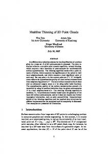
(a) Hinge: Difference of normals.
(b) Hinge: Local variation.
(c) Chair: Difference of normals.
(d) Chair: Local variation.
Fig. 4: Haar-like high-pass graph filtering based local variation (14) outperforms the DoN method. Experimental Validations. Figure 4 compares the Haarlike high-pass graph filtering based local variation (14) (second column) with that computed from the difference of normals (DoN) method (first column) [42] which is used to analyze point clouds for segmentation and contour detection. As a contour detection technique, DoN computes the difference between surface normals calculated at two scales. In each plot, we highlight the points that have top 10% largest DoN scores or local variations. In Figure 4 (a), we see that DoN cannot find the boundary in the plane because the surface normal does not change. The performance of DoN is also sensitive
8
Fig. 5: Haar-like high-pass graph filtering based local variation (14) outperforms pairwise difference based local variation (18). We use local variation to capture the contour. The first row shows the original point clouds; the second and third rows show the resampled versions with respect to two local variations: pairwise difference based local variation (18) and Haar-like high-pass graph filtering based local variation (14). Two resampled versions have the same number of points, which is 10% of points in the original point cloud.
to predeisgned radius. For example, the difference of normals cannot capture precise contours in the hinge. On the other hand, local variation captures all the contours precisely in Figure 4 (b). We see similar results in Figures 4 (c), (d), (e) and (f). Further, difference of normals needs to compute the first principle component of the neighboring points for each 3D point, which is computationally inefficient. The local variation only involves a sparse matrix and vector multiplication, which is computationally efficient. Figure 5 shows the local variation based resampling distribution on some examples of the point cloud, including hinge, cone, table, chair and trash container. The first column shows the original point clouds; the second and third rows show the resampled versions with respect to two local variations: pairwise difference based local variation (18) and Haar-like highpass graph filtering based local variation (14). Two resampled versions have the same number of points, which is 10% of points in the original point cloud. For two simulated objects, the hinge and the cone (first two rows), the pairwise difference based local variation (18) fails to detect contour and the Haar-like high-pass graph filtering based local variation (14) detects all the contours. For the real objects, the Haar-like high-pass graph filtering based resampling (14) also outperform the pairwise difference based local variation (18). In summary, the Haar-like high-pass graph filtering based local variation (14) shows the contours
of objects by using only 10% of points.
(a) Hinge with textures.
(b) Resampled version.
Fig. 6: High-pass graph filtering based resampling strategy detects both the geometric contour and the texture contour. The high-pass graph filtering based resampling strategy can be easily extended to detect transient changes in other attributes. Figure 6 (a) simulates a hinge with two different textures. The points in black have the same texture with value 0 and the points indicated by a green circle have a different texture with value 1. We put the texture as a new attribute and the point cloud matrix X ∈ RN ×4 , where the first three columns are 3D coordinates and the fourth column is the texture. We resample 10% of points based on the highpass graph filtering based local variation (14). Figure 6 (b)
9
shows the resamped point cloud, which clearly detects both the geometric contour and the texture contour. C. Low-pass Graph Filtering In classical signal processing, a low-pass filter is used to capture rough shape of a smooth signal and reduce noise. Similarly, we use a low-pass graph filter to capture rough shape of a point cloud and reduce sampling noise during resampling. Since we use the 3D coordinates of points to construct a graph (3), the 3D coordinates are naturally smooth on this graph, meaning that two adjacent points in the graph have similar coordinates in the 3D space. When a 3D point cloud is corrupted by noises and outliers, a low-pass graph filter, as a denoising operator, uses local neighboring information to approximate a true position for each point. Since the output after low-pass graph filtering is a denoised version of the original point cloud, it is more appropriate to resample from denoised points than original points. 1) Ideal low-pass graph filter: A straightforward choice is an ideal low-pass graph filter, which completely eliminates all graph frequencies above a given graph frequency while passing those below unchanged. An ideal low-pass graph filter with bandwidth b is � � Ib×b 0b×(N −b) hIL (A) = V V−1 0(N −b)×b 0(N −b)×(N −b) =
V(b) VT(b) ∈ RN ×N ,
where V(b) is the first b columns of V, and the graph frequency � response is 1, i ≤ b; hIL (λi ) = (19) 0, otherwise. The ideal low-pass graph filter hIL projects an input graph signal onto a bandlimited subspace [34] and hIL (A)s is a bandlimited approximation of the original graph signal s. We show an example in Figure 7. Figure 7 (b), (c) and (d) shows that the bandlimited approximation of the 3D coordinates of a teapot gets better when the bandwidth b increases. We see that the bandwidth influences the shape of the teapot rapidly: with ten graph frequencies, we only obtain a rough structure of the teapot. Figure 7 (e) shows that the main energy is concentrated in the low-pass graph frequency band. The feature-extraction operator f (X) = V(b) VT(b) X is shift and rotation-varying. Based on Theorem 4, the corresponding optimal resampling strategy is r � � 2
� 2
∗ c2 V(b) i 2 + V(b) VT(b) Xo (20) πi ∝ i 2 q
2 2 c2 kvi k2 + Xo T V(b) vi 2 , = where vi ∈ Rb is the ith row of V(b) . A direct way to obtain kvi k2 requires the truncated eigendecomposition (6), whose computational cost is O(N b2 ), where b is the bandwidth. It is potentially possible to approximate the leverage scores through a fast algorithm [43], [44], where we use randomized techniques to avoid the eigendecomposition and the computational cost is O(N b log(N )). Another way to leverage computation is to partition a graph into several subgraphs and obtain leverage scores in each subgraph.
2) Haar-like low-pass graph filter: Another simple choice is Haar-like low-pass graph filter; that is, 1 hHL (A) = I + A |λmax | 1 1 + |λλmax 0 | λ2 0 1 + |λmax | = V .. .. . . 0 0
(21) ··· ··· .. . ···
0 0 .. . 1+
λN |λmax |
−1 V ,
where λmax = maxi |λi | with λi eigenvalues of A. The normalization factor λmax is presented to avoid the amplification of the magnitude. We denote Anorm = A /|λmax | for simplicity. The graph frequency response is hHL (λi ) = 1+λi /|λmax |. Since the eigenvalues are ordered in a descending order, we have 1 + λi ≥ 1 + λi+1 , meaning low frequency response amplifies and high frequency response attenuates. In the graph vertex domain, the response of the ith point is P (hHL (A) X)i = xi + j∈Ni (Anorm )i,j xj , where Ni is the neighbors of the ith point. We see that hHL (A) averages the attributes of each point and its neighbors to provide a smooth output. The feature-extraction operator f (X) = hHL (A) X is shift and rotation-variant. Based on Theorem 4, the corresponding optimal resampling strategy is q 2 2 πi∗ ∝ c2 k(I + Anorm )i k2 + k((I + Anorm ) Xo )i k2 , (22) To obtain this optimal resampling distribution, we need to compute the largest magnitude eigenvalue 2 λmax , which takes O(N ), and compute k(I + Anorm )i k2 2 and k((I + Anorm ) Xo )i k2 for each row, which takes O(kvec(A)k0 ) with kvec(A)k0 the nonzero elements in the graph shift operator. We can avoid computing the largest magnitude by using a normalized adjacency matrix or a transition matrix as a graph shift operator. A normalized 1 1 adjacency matrix is D− 2 W D− 2 , where D is the diagonal degree matrix, and a transition matrix is obtained by normalizing the sum of each row of an adjacency matrix to be one; that is D−1 W. In both cases, the largest eigenvalue of a transition matrix is one, we thus have A = Anorm . Experimental Validations. We aim to use a low-pass graph filter to handle a noisy point cloud. Figure 8 (a) shows a point cloud of a fitness ball, which contains 62, 235 points collected from a Kinect device. In this noiseless case, the surface of the fitness can be modeled by a sphere. Figure 8 (b) fits a green sphere to the fitness ball 2 . The � radius and the central point of � this sphere is 0.318238 and 0.0832627 0.190267 1.1725 . To leverage the computation, we resample a subset of points and fit another sphere to the resample points. We want these two spheres generated by the original point cloud and the resampled point cloud to be similar. In many real cases, the original points are collected with noise. To simulate the noisy case, we add the Gaussian noise with mean zeros and variance 0.02 to each points. Figures 9 2 Figure
8 (b) is generated from a public software CloudCompare.
10
(a) Teapot.
(b) Approximation with 10 graph frequencies.
(c) Approximation with 100 graph frequencies.
(d) Approximation with 500 graph frequencies.
(e) Graph spectral distribution.
Fig. 7: Low-pass approximation represents the main shape of the original point clouds. Plot (a) shows a point cloud with 8, 000 points representing a teapot. Plots (b), (c) and (d) show the approximations with 10, 100 and 500 graph frequencies. We see that the approximation with 10 graph frequencies shows a rough structure of a teapot; the approximation with 100 graph frequencies can be recognized as a teapot; the approximation with 500 graph frequencies show some details of the teapot. Plot (e) shows the graph spectral distribution, which clearly shows that most energy is concentrated in the low-pass band.
Radius Center-x Center-y Center-z
Original ball (Figure 8 (a) )
Noisy ball (Figure 9 (a) )
Uniform resampling (Figure 9 (b) )
Denoised ball (Figure 9 (c) )
Low-pass graph filtering based resampling (Figure 9 (d) )
0.3182 0.0833 0.1903 1.1725
0.3478 0.0903 0.2136 1.3803
0.3520(10.6223%) 0.0975 (17.0468%) 0.1794 (5.7278%) 1.1530 (1.6631%)
0.3143 (1.2256%) 0.0799 (4.0816%) 0.1866 (1.9443%) 1.1618 (0.9126%)
0.3199 (0.5343%) 0.0849 (1.9208%) 0.1783 (6.3058%) 1.1613 (0.9552%)
(9.3023%) (8.4034%) (12.2438%) (17.7228%)
TABLE I: Proposed resampling strategy with low-pass graph filtering provides a robust shape modeling for a fitness ball. The first column is the ground truth. The relative error is shown in the parentheses. Best results are marked in bold.
(a) Fitness ball.
(b) Sphere Fitting.
Fig. 8: Shape modeling for a fitness ball. (a) and (b) show a noisy point cloud and its resampled version based on uniform resampling, respectively. Figures 9 (c) and (d) show a denoised point cloud and its resampled version, respectively. The denoised point cloud is obtained by the lowpass graph filtering (21) and the resampling strategy is based on (20). We fit a sphere to each of the four point clouds and the statistics are shown in Table I. The relative errors are shown in the parenthesis, which is defined as Error = |(x − x ˆ)/x|, where x is the ground truth, and x ˆ is the estimation. The denoised ball and its resampled version outperform the noisy ball and the uniform-sampled version because the estimated radius and the central point is closer to the original radius and the central point. This validates that the proposed resampling strategy with low-pass graph filtering provides a robust shape modeling for noisy point clouds. D. Graph Filter Banks In classical signal processing, a filter bank is an array of band-pass filters that analyze an input signal in multiple
(a) Noisy ball.
(b) Uniform resampling.
(c) Denoised ball.
(d) Low-pass graph filtering based resampling.
Fig. 9: Denoising and resampling of a noisy fitness ball. Plot (c) denoises Plot (a). Plot (d) resamples from Plot (c) according to the resampling strategy (20)
subbands and synthesize the original signal from all the subbands [45], [46]. We use a similar idea to analyze a 3D point cloud: separate an input 3D point cloud into multiple
11
All points Uniform resampling High-pass graph filtering based resampling (16)
RMSE
Errorshift
Errorrotation
4.22 4.27 1.49
8.76 9.38 0.01
2.30 × 10⁻³ 3.76 × 10⁻³ 4.29 × 10⁻⁵
TABLE II: Proposed high-pass graph filtering based resampling strategy provides an accurate registration for a sofa. Best results are marked in bold. High-pass graph filtering based resampling chooses key points and provides the best registration performance. Fig. 10: Graph filter bank analysis for 3D point clouds. In the analysis part, we separate a 3D point cloud into multiple subbands. In each subband, we resample a subset of 3D points based on a specific graph filter h(A). The number of samples in each subband is determined by a sampling ratio α. In the synthesis part, we use all the resampled points to reconstruct a surface via a reconstruction operator Φ.
components via different resampling operators, allowing us to enhance different components of a 3D point cloud. For example, we resample both contour points and noncontour points to reconstruct the original surfaces, but we need more contour points to emphasize contours. Figure 10 shows a surface reconstruction system for a 3D point cloud based on graph filter banks. In the analysis part, we separate a 3D point cloud X into k subbands. In each subband, the information preserved is determined by a specific graph filter and we resample a subset of 3D points according to (11) and (12). The number of samples in each subband is determined by a sampling ratio α. We have flexibility to use either the original 3D points or the 3D points after graph filtering. In the synthesis part, we use the resampled points to reconstruct the surface. A literature review on surface reconstruction algorithms is shown in [47]. Since each surface reconstruction algorithm has its own specific set of assumptions, different surface reconstruction algorithms perform differently on the same set of 3D points. We measure the overall performance of a surface reconstruction system by reconstruction error, which is the difference between the surface reconstructed from resampled points and the original surface. This leads to a rate-distortion like tradeoff: when we resample more points, we encode more bits and the reconstruction error is smaller; when we resample fewer points, we encode less bits and the reconstruction error is larger. The overall goal is: given an arbitrary tolerance of reconstruction error, we use as few samples as possible to reconstruct a surface by carefully choosing a graph filter and sampling ratio in each subband. Such a surface reconstruction system will benefit a 3D point cloud storage and compression because we only need to store a few resampled points. Since a surface reconstruction system is application-dependent, the design details are beyond the scope of this paper. V. A PPLICATIONS In this section, we apply the proposed resampling strategies to accurate registration. In this task, we use the proposed
resampling strategy (16) to make two point clouds registered efficiently and accurately. Figure 11 (a) shows a point cloud of a sofa, which contains 1, 204, 055 points collected from a Kinect based SLAM system [40]. As shown in Figure 11 (a), we split the original point cloud into two overlapping point clouds marked in red and blue, respectively. We intentionally shift and rotate the red part. The task is to invert the process and retrieve the shift and rotation. We use the iterative closest point (ICP) algorithm to register two point clouds, which is a standard algorithm to rotate and shift different scans into a consistent coordinate frame [48]. The ICP algorithm iteratively revises the rigid body transformation (combination of shift and rotation) needed to minimize the distance from the source to the reference point cloud. Figures 11 (b) and (c) show the registered sofa and the details of the overlapping part after registration, respectively. We see that the registration process recovers the overall structure of the original point cloud, but still leaves some mismatch in a detailed level. Since it is inefficient to register two large-scale point clouds, we want to resample a subset of 3D points from each point cloud and implement registration. We will compare the registration performance between uniformly resampled point cloud and high-pass graph filtering based resampled point cloud. Note that high-pass graph filtering based resampling can enhance the contours and key points. Figures 11 (d) and (g) show the resampled point clouds based on uniform resampling and high-pass graph filtering based resampling, respectively. Two resampled versions have the same number of points, which is 5% of points in the original point cloud. We see that Figures 11 (g) shows more contours than Figures 11 (d). Based on the uniformly resampled version Figures 11 (d), Figures 11 (e) and (f) show the registered sofa and the details of the overlapping part after registration, respectively. Based on the contour-enhanced resampled version Figures 11 (g), Figures 11 (h) and (i) show the registered sofa and the details of the overlapping part after registration, respectively. We see that the registration based on high-pass graph filtering based resampling precisely recovers the original point cloud, even in a detailed level. The intuition is that the high-pass graph filters enhance the contours, which make sharper match between the sources and targets, and thus the registration becomes easier. The quantitative results are shown in Table II, where the first column shows the root mean square error (RMSE); the second column shows the shift error; The third column shows the rotation error. Specially, RMSE =
12
(a) Original point cloud.
(b) Registered point cloud.
(c) Details.
(d) Uniform resampling (↓ 20).
(e) Registered point cloud.
(f) Details.
(g) High-pass graph filtering based graph filtering (↓ 20).
(h) Registered point cloud.
(i) Details.
Fig. 11: Accurate registration for sofa. The first row shows the original point cloud; the second row shows the uniformly resampled point cloud; and the third row shows the high-pass graph filtering based resampled point cloud (16). The first column shows the point clouds before registration; the second column shows the point clouds after registration; and the second column shows the registration details around the overlapping area. High-pass graph filtering-based resampling provides more precise registration by using fewer points. qP N
2
minj=1,...,N kb xi − xj k2 , Errorshift = kb a − ak2 and
b
b are the bi , a b and R Errorrotation = R − R , where x Frobenius 3D coordinates of the ith point, recovered shift vector and recovered rotation matrix after registration, respectively; xi , a and R are the ground-truth 3D coordinates of the ith point, ground-truth shift vector and ground-truth recovered rotation matrix. We see that high-pass graph filtering based resampled point cloud uses 20-times fewer points and achieves even better results than using all the points. The shift and rotation errors of using high-pass graph filtering based resampling are significantly smaller than those of using all the points or using uniform resampling. i=1
VI. C ONCLUSIONS In this paper, we proposed a resampling framework to select a subset of points to extract application-dependent features and reduce the subsequent computation in a large-scale point cloud. We formulated an optimization problem to obtain the optimal resampling distribution, which is also guaranteed to be shift/rotation/scale invariant. We then specified the feature extraction operator to be a graph filter and studied the resampling strategies based on all-pass, low-pass and high-pass graph filtering. A surface reconstruction system based on graph filter banks was introduced to compress 3D point clouds. Three applications, including large-scale visualization, accurate registration and robust shape modeling, were presented to validate the effectiveness and efficiency of the proposed resampling methods. This work also pointed out many possible future
directions of 3D point cloud processing, such as efficient 3D point cloud compression system based on graph filter banks, surface reconstruction based on arbitrary graphs, robust metric to evaluate the quality of a 3D point cloud. R EFERENCES [1] R. B. Rusu and S. Cousins, “3D is here: Point cloud library (PCL),” in IEEE International Conference on Robotics and Automation (ICRA), Shanghai, CN, May 2011. [2] H. Hoppe, T. DeRose, T. Duchamp, J. McDonald, and W. Stuetzle, “Surface reconstruction from unorganized points,” ACM Trans. Graph. Proceedings of ACM SIGGRAPH, vol. 26, pp. 71–78, Jul. 1992. [3] J. Kammerl, N. Blodow, R. B. Rusu, S. Gedikli, M. Beetz, and E. Steinbach, “Real-time compression of point cloud streams,” in Robotics and Automation (ICRA), 2012 IEEE International Conference on, St. Paul, MN, USA, May 2012, pp. 778–785. [4] C. Zhang, D. Florencio, and C. T. Loop, “Point cloud attribute compression with graph transform,” in Proc. IEEE Int. Conf. Image Process., Paris, France, Oct. 2014, pp. 2066–2070. [5] D. Thanou, P. A. Chou, and P. Frossard, “Graph-based compression of dynamic 3d point cloud sequences,” IEEE Trans. Image Process., vol. 25, no. 4, pp. 1765–1778, Feb. 2016. [6] A. Anis, P. A. Chou, and A. Ortega, “Compression of dynamic 3d point clouds using subdivisional meshes and graph wavelet transforms,” in 2016 IEEE International Conference on Acoustics, Speech and Signal Processing, ICASSP 2016, Shanghai, China, March 20-25, 2016, 2016, pp. 6360–6364. [7] P. Oesterling, C. Heine, H. J¨anicke, G. Scheuermann, and G. Heyer, “Visualization of high-dimensional point clouds using their density distribution’s topology,” IEEE Trans. Vis. Comput. Graph., vol. 17, no. 11, pp. 1547–1559, 2011. [8] S. Pecnik, D. Mongus, and B. Zalik, “Evaluation of optimized visualization of lidar point clouds, based on visual perception,” in Human-Computer Interaction and Knowledge Discovery in Complex, Unstructured, Big Data (HCI-KDD), Maribor, Slovenia, Jul. 2013, pp. 366–385.
13
[9] B. F. Gregorski, B. Hamann, and K. I. Joy, “Reconstruction of bspline surfaces from scattered data points,” in Computer Graphics International, Geneva, Switzerland, Jun. 2000, pp. 163–170. [10] A. Golovinskiy, V. G. Kim, and T. A. Funkhouser, “Shape-based recognition of 3d point clouds in urban environments,” in Proc. IEEE Int. Conf. Comput. Vis., Kyoto, Japan, Sep. 2009, pp. 2154–2161. [11] M. Alexa, J. Behr, D. Cohen-Or, S. Fleishman, D. Levin, and C. T. Silva, “Computing and rendering point set surfaces,” IEEE Trans. on Visualization and Computer Graphics, vol. 9, pp. 3–15, Jan. 2003. [12] F. Ryden, S. N. Kosari, and H. J. Chizeck, “Proxy method for fast haptic rendering from time varying point clouds,” in IEEE/RSJ International Conference on Intelligent Robots and Systems, IROS, San Francisco, CA, Sep. 2011, pp. 2614–2619. [13] I. Guskov, W. Sweldens, and P. Schr¨oder, “Multiresolution signal processing for meshes,” Proceedings of SIGGRAPH, vol. 24, no. 3, pp. 325–334, July 1999. [14] M. Wand, A. Berner, M. Bokeloh, A. Fleck, M. Hoffmann, P. Jenke, B. Maier, D. Staneker, and A. Schilling, “Interactive editing of large point clouds,” in Symposium on Point Based Graphics, Prague, Czech Republic, 2007, pp. 37–45. [15] K. Demarsin, D. Vanderstraeten, T. Volodine, and D. Roose, “Detection of closed sharp feature lines in point clouds for reverse engineering applications,” in Geometric Modeling and Processing, Pittsburgh, PA, 2006, pp. 571–577. [16] C. Weber, S. Hahmann, and H. Hagen, “Sharp feature detection in point clouds,” in Shape Modeling International Conference, Aix en Provence, France, Jun. 2010, pp. 175–186. [17] J. Daniels, L. K. Ha, T. Ochotta, and C. T. Silva, “Robust smooth feature extraction from point clouds,” in Shape Modeling and Applications, 2007. SMI’07. IEEE International Conference on, Lyon, France, June 2007, IEEE, pp. 123–136. [18] C. Choi, A. J. Trevor, and H.I. Christensen, “Rgb-d edge detection and edge-based registration,” in 2013 IEEE/RSJ International Conference on Intelligent Robots and Systems, Tokyo, Japan, Nov. 2013, IEEE, pp. 1568–1575. [19] C. Feng, Y. Taguchi, and V. Kamat, “Fast plane extraction in organized point clouds using agglomerative hierarchical clustering,” in Proceedings of IEEE International Conference on Robotics and Automation, Hong Kong, May 2014, pp. 6218–6225. [20] M. Shahzad and X. Zhu, “Robust reconstruction of building facades for large areas using spaceborne tomosar point clouds,” IEEE Trans. Geoscience and Remote Sensing, vol. 53, no. 2, pp. 752–769, 2015. [21] W. Luo and H. Zhang, “Visual analysis of large-scale lidar point clouds,” in IEEE International Conference on Big Data, Santa Clara, CA, Nov. 2015, pp. 2487–2492. [22] J. Ryde and H. Hu, “3D mapping with multi-resolution occupied voxel lists,” Autonomous Robots, pp. 169–185, Apr. 2010. [23] C. T. Loop, C. Zhang, and Z. Zhang, “Real-time high-resolution sparse voxelization with application to image-based modeling,” in Proceedings of the 5th High-Performance Graphics 2013 Conference HPG ’13, Anaheim, California, USA, July 2013, pp. 73–80. [24] J. Peng and C.-C. Jay Kuo, “Geometry-guided progressive lossless 3D mesh coding with octree (OT) decomposition,” ACM Trans. Graph. Proceedings of ACM SIGGRAPH, vol. 24, no. 3, pp. 609–616, Jul. 2005. [25] A. Hornung, K. M. Wurm, M. Bennewitz, C. Stachniss, and W. Burgard, “Octomap: An efficient probabilistic 3D mapping framework based on octrees,” Autonomous Robots, pp. 189–206, Apr. 2013. [26] B. Eckart and A. Kelly, “Rem-seg: A robust em algorithm for parallel segmentation and registration of point clouds,” in IEEE/RSJ International Conference on Intelligent Robots and Systems, Tokyo, Japan, Jun. 2013, pp. 4355–4362. [27] B. Eckart, K. Kim, A. Troccoli, A. Kelly, and J. Kautz, “Accelerated generative models for 3D point cloud data,” in Proc. IEEE Int. Conf. Comput. Vis. Pattern Recogn., Las Vegas, Nevada, Jun. 2016. [28] J. Peng, C-S. Kim, and C.-C. Jay Kuo, “Technologies for 3D mesh compression: A survey,” J. Vis. Comun. Image Represent., vol. 16, no. 6, pp. 688–733, Dec. 2005. [29] P. Alliez and C. Gotsman, “Recent advances in compression of 3D meshes,” in In Advances in Multiresolution for Geometric Modelling. 2003, pp. 3–26, Springer-Verlag. [30] A. Maglo, G. Lavou´e, F. Dupont, and C. Hudelot, “3D mesh compression: Survey, comparisons, and emerging trends,” ACM Comput. Surv., vol. 47, no. 3, pp. 44:1–44:41, Feb. 2015. [31] T. Hackel, J. D. Wegner, and K. Schindler, “Contour detection in unstructured 3d point clouds,” in Proc. IEEE Int. Conf. Comput. Vis. Pattern Recogn., Las Vegas, Nevada, Jun. 2016.
[32] A. Sandryhaila and J. M. F. Moura, “Discrete signal processing on graphs,” IEEE Trans. Signal Process., vol. 61, no. 7, pp. 1644–1656, Apr. 2013. [33] D. I. Shuman, S. K. Narang, P. Frossard, A. Ortega, and P. Vandergheynst, “The emerging field of signal processing on graphs: Extending high-dimensional data analysis to networks and other irregular domains,” IEEE Signal Process. Mag., vol. 30, pp. 83–98, May 2013. [34] S. Chen, R. Varma, A. Sandryhaila, and J. Kovaˇcevi´c, “Discrete signal processing on graphs: Sampling theory,” IEEE Trans. Signal Process., vol. 63, no. 24, pp. 6510–6523, Dec. 2015. [35] A. Anis, A. Gadde, and A. Ortega, “Efficient sampling set selection for bandlimited graph signals using graph spectral proxies,” IEEE Trans. Signal Process., vol. 64, pp. 3775–3789, July 2016. [36] A. G. Marques, S. Segarra, G. Leus, and A. Ribeiro, “Sampling of graph signals with successive local aggregations,” IEEE Trans. Signal Process., vol. 64, pp. 1832 – 1843, 2015. [37] M. Tsitsvero, S. Barbarossa, and P. D. Lorenzo, “Signals on graphs: Uncertainty principle and sampling,” IEEE Trans. Signal Process., vol. 64, pp. 4845 – 4860, 2015. [38] L. D. Floriani and P. Magillo, “Multiresolution mesh representation: Models and data structures,” in Tutorials on Multiresolution in Geometric Modelling, Summer School Lecture Notes, pp. 363–417. Springer, 2002. [39] A. Sandryhaila and J. M. F. Moura, “Discrete signal processing on graphs: Frequency analysis,” IEEE Trans. Signal Process., vol. 62, no. 12, pp. 3042–3054, June 2014. [40] Y. Taguchi, Y-D Jian, S. Ramalingam, and C. Feng, “Point-plane slam for hand-held 3d sensors,” in Proceedings of IEEE International Conference on Robotics and Automation, Karlsruhe, May 2013. [41] D. K. Hammond, P. Vandergheynst, and R. Gribonval, “Wavelets on graphs via spectral graph theory,” Appl. Comput. Harmon. Anal., vol. 30, pp. 129–150, Mar. 2011. [42] Y. Loannou, B. Taati, R. Harrap, and M. A. Greenspan, “Difference of normals as a multi-scale operator in unorganized point clouds,” in 2012 Second International Conference on 3D Imaging, Modeling, Processing, Visualization & Transmission, Zurich, Switzerland, October 13-15, 2012, 2012, pp. 501–508. [43] P. Drineas, M. Magdon-Ismail, M. W. Mahoney, and D. Woodruff, “Fast approximation of matrix coherence and statistical leverage,” J. Mach. Learn. Res., vol. 13, no. 1, pp. 3475–3506, 2012. [44] D. P. Woodruff, “Sketching as a tool for numerical linear algebra,” Foundations and Trends in Theoretical Computer Science, vol. 10, pp. 1–157, Oct. 2014. [45] M. Vetterli, J. Kovaˇcevi´c, and V. K. Goyal, Foundations of Signal Processing, Cambridge University Press, Cambridge, 2014, http://foundationsofsignalprocessing.org. [46] J. Kovaˇcevi´c, V. K. Goyal, and M. Vetterli, Fourier and Wavelet Signal Processing, Cambridge University Press, Cambridge, 2016, http://www.fourierandwavelets.org/. [47] M. Berger, A. Tagliasacchi, L. M. Seversky, P. Alliez, G. Guennebaud, J. A. Levine, A. Sharf, and C. T. Silva, “A survey of surface reconstruction from point clouds,” Computer Graphics Forum, 2016. [48] P. J. Besl and N. D. McKay, “A method for registration of 3-d shapes,” IEEE Trans. Pattern Anal. Mach. Intell., vol. 14, no. 2, pp. 239–256, 1992. [49] M. Kazhdan, M. Bolitho, and H. Hoppe, “Poisson surface reconstruction,” in Proceedings of the fourth Eurographics symposium on Geometry processing, 2006, vol. 7.
A PPENDIX A. Proof of Lemma 1 Proof. For the nonweighted version, we have X � EΨ∼π ΨT Ψf (X) i = EM fMj (X)δMj =i Mj ∈M (a)
=
M E` (f` (X)δ`=i ) = M
N X
f` (X)π` δ`=i
`=1
=
M πi fi (X).
� where ΨT Ψf (X) i ∈ RK is the ith row of ΨT Ψf (X), fi (X) ∈ RK is the ith row of f (X), δi denotes an indicator
14
function and equality (a) follows from the independent and identically distributed random sampling. For the reweighted version, we have
C. Proof of Theorem 2 Proof. Based on Theorem 1, we have EΨ∼π (Df (Ψ))
EΨ∼π =
EM
T
� S Ψ Ψf (X) i
= EΨ∼π
X
= EΨ∼π
SMj ,Mj fMj (X)δMj =i
� =
M E`
=
fi (X).
1 f` (X)δ`=i M πl
� = M
N X `=1
1 f` (X)π` δ`=i M π`
� �
S ΨT Ψ − I f X0c
max 0
� �
S ΨT Ψ − I F X0c
X0c :kXc k2 =c X0 :kXc k2 =c
�c
Mj ∈M
max 0
�� 2 Xo F � 2 Xo F
�
S ΨT Ψ − I F X0c 2 F X0c :kXc k2 =c �
2 � + S ΨT Ψ − I F Xo F �
� 2 = EΨ∼π c2 S ΨT Ψ − I F F �
2 � T
+ S Ψ Ψ − I F Xo F � � = c2 Tr F Q FT + Tr F Xo Q(F Xo )T .
= EΨ∼π
max 0
B. Proof of Theorem 1 Proof. We first split the error into the bias term and the variance term,
2 EΨ∼π S ΨT Ψf (X) − f (X) 2
2 � = EΨ∼π S ΨT Ψf (X) − f (X) 2
� 2 +EΨ∼π S ΨT Ψf (X) − EΨ∼π S ΨT Ψf (X) 2 , where the first term is bias and the second term is variance. Lemma (1) shows that the bias term is zero. So, we only need to bound the variance term. For each element in the variance term, we have
=
� � 2 EΨ∼π S ΨT Ψf (X) i − E S ΨT Ψf (X) i T " X EM SMj ,Mj fMj (X)δMj =i − fi (X) Mj ∈M
X
� min EΨ∼π Df (X) (Ψ)
(23)
π
subject to
N X
πi ≥ 0.
πi = 1,
i=1
The corresponding Lagrange function is L(πi , λ, µ) = EΨ∼π
N X � Df (X) (Ψ) + λ πi − 1
! +
i=1
N X
µi πi
i=1
! � N � N N X X X 1 2 = µi πi , − 1 kfi (X)k2 + λ πi − 1 + πi i=1 i=1 i=1
where the equality follows from Theorem 1. The derivative to πi is ∂L 1 2 = − 2 kfi (X)k2 + λ + µi . (24) fMj (X)T fMj0 (X) ∂πi πi
SMj0 ,Mj0 fMj0 (X)δMj0 =i − fi (X)
Mj 0 ∈M
= EM
Proof. The optimal resampling strategy is the solution of the following optimization problem,
#
�
D. Proof of Theorem 3
X
SMj ,Mj SMj0 ,Mj0
Mj ,Mj 0 ∈M
� δMj =i δMj0 =i
− fi (X)T fi (X)
= M 2 E` S2`,` f` (X)T f` (X)δ`=i − fi (X)T fi (X) = M2 � =
N X f` (X)T f` (X)
M 2 π`2
π` δ`=i − fi (X)T fi (X)
`=1 � 1 − 1 fi (X)T fi (X). πi
We finally combine all the elements and obtain (8).
By setting its derivative to zero, we have kfi (X)k2 . πi = √ λ + µi Due to the complementary slackness, we have µi πi =
µi kfi (X)k2 √ = 0. λ + µi
Thus, either µi or kfi (X)k2 is zero. In both cases, πi ∝ kfi (X)k2 .
15
E. Proof of Theorem 4 Proof. The optimal resampling strategy is the solution of the following optimization problem, min EΨ∼π (Df (Ψ))
(25)
π
subject to
N X
πi ≥ 0.
πi = 1,
i=1
The corresponding Lagrange function is L(πi , λ, µ) = EΨ∼π (Df (Ψ)) + µ
N X
! πi − 1
i=1
+
N X
µi πi
i=1
� � N � N � X X 1 1 2 2 − 1 kFi k2 + − 1 k(F Xo )i k2 = c π π i i i=1 i=1 ! N N X X πi − 1 + +µ µi πi , 2
i=1
i=1
where Fi is the ith row of F and (F Xo )i is the ith row of F Xo . The derivative to πi is � ∂L 1 � 2 2 = − 2 c2 kFi k2 + k(F Xo )i k2 + µ + µi . ∂πi πi By setting its derivative to zero, we have q 2 2 c2 kFi k2 + k(F Xo )i k2 √ πi = . µ + µi Due to the complementary slackness, we have q 2 2 µi c2 kFi k2 + k(F Xo )i k2 √ µi πi = = 0. µ + µi Thus, either µi or kfi (X)k2 is zero. In both cases, πi ∝ q 2 2 c2 kFi k2 + k(F Xo )i k2 . F. Proof of Theorem 5 Proof. We first show the rotational invariance. Let X be the 3D coordinates of an original point cloud and R ∈ R3×3 be a rotation matrix. The point cloud after rotating is X R. The local variation of X R is fi (X R)
2
=
k(h(A) X R)i k2
=
k(h(A))i X Rk2
=
(h(A))i X R RT XT (h(A))i
(a)
=
(h(A))i X XT (h(A))i
=
2 k(h(A) X)i k2
2 T
T
= fi (X),
where (h(A))i is the ith row of h(A) and (a) follows from any rotation matrix R is orthonormal. We next show the shift variance. Let a ∈ R3 be the shift and the point cloud after shifting is X +1aT . The local variation of X +1aT is
� �
� 2 T T
fi (X +1a ) = h(A) X +1a
i 2
� � � � 2
T
= h(A) X + h(A)1a
i
i 2
Thus, fi (X +1aT ) = fi (X) only when h(A)1 = 0 ∈ RN .