Fault architecture and related distribution of physical properties ... - Csic

ISSN: 1698-6180 www.ucm.es/info/estratig/journal.htm Journal of Iberian Geology 32 (1) 2006: 95-112

Fault architecture and related distribution of physical properties in granitic massifs: geological and geophysical methodologies Arquitectura de fallas y distribución de propiedades físicas relacionadas en macizos graníticos: metodologías geológicas y geofísicas D. Martí1*, J. Escuder Viruete2, R. Carbonell1, I. Flecha1, A. Pérez-Estaún1 (1) (2)

Instituto de Ciencias de la Tierra Jaume Almera, CSIC, Lluís Solé i Sabarís s/n, 08028 Barcelona (Spain) Departamento de Petrología y Geoquímica, Universidad Complutense de Madrid, 28040 Madrid (Spain) *Corresponding author: [email protected] Received: 20/07/05 / Accepted: 25/09/05

Abstract Geological and geophysical data acquired in several projects aimed to characterization of structures in granitic rocks, make possible to evaluate the efficiency and resolution of several geological and geophysical methodologies for their study. The analysis of the spatial distribution of fracture density in granitic bodies makes possible to identify fault damage zones as well as the central fault cores. Measures of Fracture Index in a granitic massif can be used to generate 3-D stochastic models and simulations, which provide an image of the architecture of fault zones and the related distribution of physical properties. Geostatistical methods are a tool to integrate geological and geophysical data in 3-D. Borehole and surface geophysical data provide additional constraints for fracture mapping of a granitic body. High resolution reflection seismic experiments together with azimut variable vertical seismic profiles acquired in borehole, as well as surface tomographic 3-D acquisition, have proved to be very efficient in resolving the fault structure of granites. Keywords: Fault zone, fault zone architecture, geostatistical modeling, seismic velocities, seismic tomography, seismic anisotropy. Resumen El desarrollo de varios proyectos para la caracterización de macizos graníticos nos ha permitido evaluar la capacidad de resolución y eficacia de diversas metodologías de trabajo geológicas y geofísicas. La distribución espacial de la densidad de fracturación en macizos graníticos permite identificar el núcleo de las zonas de falla y las áreas dañadas de su entorno. Medidas del índice de fracturación procedentes de la superficie y de los sondeos, pueden ser usadas para generar modelos 3-D estocásticos que proporcionan una imagen de la arquitectura de las zonas de falla y la distribución de propiedades físicas en el cuerpo granítico. Los métodos geoestadísticos proporcionan la posibilidad de integrar los datos geológicos y geofísicos para visualizar la distribución de fracturas en el macizo rocoso. Experimentos de sísmica de reflexión de alta resolución, junto con perfiles sísmicos verticales adquiridos en sondeos con azimut variable y experimentos tomográficos 3-D adquiridos en superficie, han demostrado ser metodologías válidas para resolver la estructura interior de los granitos. Palabras clave: Zona de falla, arquitectura de las zonas de falla, modelado geostadístico, velocidades sísmicas, tomografía sísmica, anisotropía sísmica.

96

Martí et al. / Journal of Iberian Geology 32 (1) 2006: 95-112

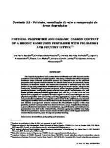
1. Introduction Fault zones generated in brittle conditions are lithologically heterogeneous and structurally anisotropic discontinuities in the upper crust. Resolving the mesoscopic structure of fault zones at scales between one centimeter and hundreds of meters is important for a variety of applications, which include: hydrogeology, hydrocarbon migration, toxic and non-toxic waste isolation, ore deposits, earthquake nucleation and propagation, paleoseismology, and the rheological/mechanical behavior of faults (Barton et al., 1988; Forster and Evans, 1991; Bruhn et al., 1994; Caine et al. 1996; Fisher and Knipe, 1998; Li et al., 1998; Schulz and Evans, 1998, 2000). The influence of fault zones on permeability, fluid flow, chemical changes and fluid-flow interactions in crystalline massifs has been widely recognized (Barton et al., 1988; Scholz and Anders, 1994; Goddard and Evans, 1995; Caine et al., 1996; Schulz and Evans, 1998, 2000). The objective of this contribution is to analyze some geological and geophysical methodologies to be used to determine fault zones architecture and the distribution of related physical properties within a granitic massif. Faults can be divided into two distinct components: the fault core, where most of the displacement is accommodated, and the damaged zone (Fig. 1), that is mechanically related to the growth of the fault zone (Sibson, 1977;

Chester and Logan, 1987; Smith et al., 1990; Forster and Evans, 1991; Caine et al., 1993; 1996; Scholz and Anders, 1994). Fault core materials are commonly composed of one or more structural elements such as anastomosing slip surfaces, clay-rich gouge, cataclasite and fault breccias. The damage zone structures are mechanically related fracture sets, small faults, veins and joints at a variety of scales. The fault core and the damage zones are surrounded by relatively undeformed protolith. The relative shapes and sizes of each of these structural elements will vary from fault to fault and within a fault system, and there may be more than one fault core or principal slip surface within a fault zone (Chester and Logan, 1987; Chester et al., 1993; Evans and Chester, 1995; Schulz and Evans, 1998, 2000). From a lithologic, structural and hydrogeological point of view, fault core, damage zone and undeformed protolith are distinct units that reflect the material properties and deformation conditions within a fault zone (Caine et al., 1996; Schulz and Evans, 1998; 2000). This architecture controls the physical properties of fault zones (Barton et al., 1988; Bruhn et al., 1994; Evans and Chester, 1995; Wintsch et al., 1995; Evans et al., 1997; Unsworth et al., 1997; Schulz and Evans, 1998). Fault zones are only partly accessible to direct observations and, for this reason, a wide variety of geophysical methods have been used to image fault zones and related

Fig. 1.- (a) Model of fault zone architecture (after Smith et al., 1990; Caine et al., 1996). (b) Granitic massif discretization in small volumes (3-D grid) with a given value of the Fracture Index (FI) from geostatistical modeling. Fig. 1.- (a) Modelo conceptual de la arquitectura de una zona de falla (según Smith et al., 1990; Caine et al., 1996). (b) División de un macizo granítico en pequeños volúmenes (red 3-D) con diferentes valores del Índice de Fracturación (FI) del modelado geostadístico.

Martí et al. / Journal of Iberian Geology 32 (1) 2006: 95-112

97

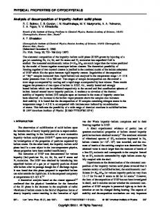
Fig. 2.- Relationships between Fracture Index (FI), P-wave velocities (VP in km/s), and S-wave velocities (VS in km/s) in the SR-3 borehole at Mina Ratones region (Albalá granitic pluton; Cáceres, Spain). Fig. 2.- Relación entre el Índice de Fracturación (FI), las velocidades de las ondas P (VP en km/s) y de las ondas S (VS en km/s) en el sondeo SR-3 de la zona de Mina Ratones (plutón de Albalá, Cáceres, España)

brittle strain. Available information of the shallow subsurface is commonly limited to one-dimensional (1-D) data arrays (core descriptions and geophysical well logs) and continuous two-dimensional (2-D) vertical seismic profiles, or other 2-D geophysical data, which generally have vertical and horizontal resolutions generally no better than of 5 and 25 m, respectively. Reflection seismics integrates surface studies with borehole results to locate low to middle-dip fault zones, some of which may be hydraulically conductive. Problems still exist when attempting to image 3-D structure in crystalline rock from 2-D acquisition geometries, where numerous out of plane reflections result. In order to properly image these structures seismic tomography and 3-D seismic data acquisition and processing are required. Fault zones in granitic rocks have different physical properties than the surrounding host rock. The presence of minor fractures, adjacent geochemically altered material and fluids (water) result in lower seismic velocities in the fault zones than in the fresh unfractured granite located

between them (Moos and Marion, 1994) (Fig. 2). Therefore, a carefully designed seismic tomography experiment should be able to map velocity differences within the granitic massif in 3-D. Shallow seismic tomography has been successful in identifying shapes and sizes of colluvial wedges (Morey and Schuster, 1999). Theoretical calculations and high resolution seismics (Kanasewich et al., 1983; Holliger and Robertsson, 1998) have shown that the shallow subsurface is a medium where most of the wave conversions take place and where seismic velocities have the largest variations. These large variations in physical properties and geometry result in a complex wavefield which makes high resolution seismic reflection images difficult to interpret. 3-D high resolution seismic reflection surveys require a considerable field effort, and are very expensive with the present technology. Recent studies developed in granites (Ratones and Iberseis projects, Barcelona Subway test) as part of ENRESA leading edge scientific research programme, have allowed us to evaluate how a fault zone may be geologi-

98

Martí et al. / Journal of Iberian Geology 32 (1) 2006: 95-112

Fig. 3.- Geological cross section of the North fault at Mina Ratones region. a, b, c, d, and e: lower hemispheric stereographic projections of mesoscopic faults and dykes observed in surface outcrops near the North Fault. f and g: rose diagrams of Cenozoic faults in the whole Mina Ratones area. h: lower hemispheric stereographic projections of North Fault related faults from SR-2 well core. i: paleostress analysis carried out on Cenozoic faults. From Escuder Viruete et al. (2004). Fig. 3.- Corte geológico mostrando la Falla Norte en la región de Mina Ratones. a, b, c, d, y e: proyección estereográfica en el hemisferio inferior de fallas mesoscópicas y diques medidos en superficie cerca de la Falla Norte. f and g: diagramas en rosa de las fallas Cenozoicas del entorno de Mina Ratones. h: proyección estreográfica en el hemisferio inferior de las fallas relacionadas con la Falla Norte, medidas en el sondeo SR-2. i: análisis de “paleostress“ realizado en fallas Cenozoicas. Según Escuder Viruete et al. (2004).

cally defined in base to a combination of the distribution fault-related rocks, brittle structures, deformation mechanisms, whole-rock geochemistry, changes in physical properties, and how can be imaged at several scales by direct and indirect geophysical methods. Fracture density, structural data and fault-rock type evolution along

the damage zone, as well as geochemical, microstructural and mineralogical variations within the fault zone were recorded from field studies and boreholes (Fig. 2). Welllog data in conjunction with different seismic methodologies allow to image the fault zones architecture in a granitic massif. The results of these analyses were correlated

Martí et al. / Journal of Iberian Geology 32 (1) 2006: 95-112

99

and integrated using geostatistical modeling techniques, which permit to develop 3-D cuantitative models of fault zones distribution and related physical properties in a scale suitable for subsequent fluid flow simulations. This paper presents a synthesis of these results. 2. Geological methodologies Fault zone distribution in granitic rocks can be established on the basis of field geology, structural analysis, seismic experiments, drilled cores and sonic well-log data. An example of application of these methodologies has been done in the Ratones Project, a multidisciplinary experiment developed to evaluate the environmental impact produced by an old Uranium mine. The main results can be found in Escuder Viruete and Pérez-Estaún (1998), Carbonell et al. (1999), Escuder Viruete (1999), Jurado (1999), Escuder Viruete et al. (2001, 2003a, b), Martí et al. (2002a, b) and Pérez Estaún et al. (2002). Classical structural geology methodologies should be applied to study fracture systems in granitic massifs, including structural mapping at reliable scales. These studies comprise: geometric and cinematic analyses of fault zones, paleostress determinations (i.e., Etchecopar et al., 1981), evolution of microstructures and textures present in fault-rocks (i.e., Sibson, 1981; Parry et al., 1988, 1998), and the mineralogical and geochemical characterization of altered rocks along fault surfaces (i.e., Scholz and Anders, 1994; Caine et al., 1996) (Fig. 3). Further, the geostatistical analyses in 3-D of geological or geophysical data, as fracture density or seismic velocities, have proved to be very efficient in determining the fault zones architecture of a granitic massif. 2.1. Fracture density An observed fact in many fault zones is that fracture density in the fault damage zone increases to the central fault core (Sibson, 1977; Hancock, 1985; Goddard and Evans, 1995; Schulz and Evans, 2000). This fracture density can be quantitatively defined by a Fracture Index (FI, in m-1 units), or number of structural discontinuities existing by unit length (La Pointe and Hudson, 1985; Narr and Suppe, 1991; Engelder et al., 1997; Escuder Viruete et al., 2001). Based on the presence of a fracture density gradient perpendicular to a fault zone, FI estimates in discrete domains can be used to characterize fault zone architecture and its spatial variability using geostatistical methods. For example, Escuder Viruete et al. (2001) describe that relatively high FI values measured in outcrops are often adjacent to other relatively high FI areas,

Fig. 4.- Variogram volume and experimental variograms (from Escuder Viruete et al., 2003a). (a) three orthogonal slices through the center of symmetry of the variogram volume displaying the variogram values computed along all directions and for all available separation lags. The direction of the maximum correlation of the Fracture Index (FI) projects on the three slices along the longest axis of the central gray ellipses (black arrows) defined by the lowest values of γ(h) as a function of the separation vector. (b) Experimental variogram computed along a specific direction (45º), or directional variogram. The squares are data points of the experimental variograms, whereas the continuous line is the nested fitted model of variogram (Pannatier, 1996). The variogram model consists in an exponential structure of correlation and has a range a and a sill value of c. Fig. 4.- Variograma de volumen y variogramas experimentales (según Escuder Viruete et al., 2003a). (a) secciones ortogonales a través del centro de simetría del variograma de volumen, mostrando los valores medidos en todas las direcciones. La dirección de máxima correlación del Índice de Fracturación (FI) queda proyectada en las tres secciones a lo largo de los ejes mayores de las elipses (flechas negras) definidos por los menores valores de γ(h) como una función del vector de separación. (b) Variograma experimental calculado para una dirección específica (45º), o variograma direccional. Los cuadros son los puntos obtenidos del variograma experimental, mientras que la línea continua es la obtenida del modelo de variograma (Pannatier, 1996). El modelo de variograma consiste en una estructura exponencial de correlación que tiene un rango a y un valor del sill de c.

while low FI values cluster next to each other. High FI areas correspond with zones where fractures cluster next to each other, typical of fault damage zones, and define 2D elongated bands parallel and coincident with the traces of mapped faults. In the Mina Ratones area, FI values were estimated in several surface outcrops and in two drilled subvertical cores. FI is in the last case the number of structural discontinuities present by unit length along

Martí et al. / Journal of Iberian Geology 32 (1) 2006: 95-112

100

Fig. 5.- Interpreted relationships between fault architecture and the 3-D grid (pixel-map) of the FI in the Mina Ratones area, obtained from geostatistical simulation, looking from the SE. Fig. 5.- Interpretación de las relaciones entre la arquitectura de las fallas y la red 3-D de FI en el área de Mina Ratones, obtenida con simulación geostadística, visión desde el SE.

the well-axis. BHTV (Borehole Televiewer) images make possible to discriminate the tectonic fractures from the fractures induced as a consequence of core perforation and extraction. 2.2. Variogram modeling Fracture density is not only to be high in a damage zone, it will also be highly variable in detail in many cases (Schulz and Evans, 1998, 2000). However, as it is shown in the conceptual model of figure 1, if the damage zone-fault core of the elongated fault zones and the surrounding undeformed protolith are divided into many small individual cubes, the average FI of each cube is related with that of the surrounding cubes. The closer two cubes are to each other, the higher the probability that the FI values are similar. The aim of geostatistics is to describe this kind of spatial correlation to allow the prediction of non-measured values. Geostatistics assumes that natural variations can be described by a random, spatially correlated function. By making this assumption, a geostatistical approach is able to avoid the difficult task of reconstructing the exact process that influenced the parameter value at each location. From this approach, a semi-variogram function is used (Fig. 4) (Isaaks and Srivastava, 1989; Deutsch and Journel, 1992; Cassiraga and Gómez Hernández, 1996; Pannatier, 1996). For a set of n spatially distributed measurements of a property

(z), the semi-variogram considers all N pairs of measurements (zi, zi+h) separated from each other by a distance h. The semi-variogram value γ(h), for a separation distance h, is calculated by the sum over all [zi- zi+h] pairs located at distance h from each other: (1) γ(h) = [1/2N(h)] Σi=1…N(h) [ zi – zi+h ]2

The sample variogram is obtained by plotting all the intervals of class h versus the value of the semivariance γ(h) calculated in each interval (Isaaks and Srivastava, 1989). If a spatial correlation exists between the data, typical variograms are convex curves where it is possible to extract several parameters that define the spatial continuity model of the property (Fig. 4) (Isaaks and Srivastava, 1989; Deutsch and Journel, 1992; Cassiraga and Gómez Hernández, 1996; Pannatier, 1996). This spatial continuity model can be used to estimate the values of the property in points, cells or blocks, in one, two or threedimensions (1, 2 or 3-D). If the statistical characteristics of a geological unit are known from a set of spatially distributed data, unknown values for unmeasured points can be inferred so that the estimated unknown values also reproduce the unit’s statistical characteristics. In granitic rocks, for example, where in situ fracture density cannot be fully determined in 3-D, inferences about fault zone architecture cannot be made directly. Instead, numerical simulations allow for the synthesis of FI stochastic fields with specified statisti-

Martí et al. / Journal of Iberian Geology 32 (1) 2006: 95-112

101

Fig. 6.- P-wave velocity log from SR-5 borehole at Mina Ratones area (Albalá pluton), and statistical distribution of P-wave seismic velocities for two segments: a) from 0 to 170 m; b) from 250 to 500 m. The shallower segment (a) features a high variability with a mean value of 5.17 km/s, while the deeper segment (b) shows a narrower distribution of the velocities with a higher mean value of 5.52 km/s. The shallower segment corresponds to a fractured granite, while the lower segment is more representative of a more unfractured granite. Fig. 6.- Registro de velocidades P del sondeo SR-5 en el área de Mina Ratones (plutón de Albalá) y distribución estadística de velocidades P en dos segmentos del sondeo: a) desde 0 a 170 m; b) desde 250 a 500 m. El segmento más superficial (a) muestra una alta variabilidad, con un valor medio de 5,17 km/s, mientras que el segmento más profundo (b) muestra una distribución más estrecha con un valor medio de 5,52 km/s. La parte superior del sondeo corresponde a un granito muy fracturado, mientras que la parte baja es representativa de un granito poco fracturado.

cal characteristics. The numerical synthesis of stochastic fields of fracture density requires specification of the mean, standard deviation, variance and spatial correlation of the data (variogram function). Currently, it is assumed that these properties do not vary with time. The manner as the variogram function changes with direction and increasing distance is specified selecting an anisotropic variogram model. The resulting stochastic fracture intensity fields are used to build 3-D models of distribution of physical properties related to fault zones, or simulation of mass-transport processes, and the resulting numerical predictions about structural, geochemical or mineralogical distributions can be compared with field-based observations.

2.3. Geostatistical methodology and data collection The methodology applied to model the spatial distribution of fault zones has several steps, which are typical in any geostatistical analyses (Deutsch and Journel, 1992; Pannatier, 1996; Goovarest, 1997; Pebesma and Wesseling, 1998; Kupfersberger and Deutsch, 1999). The first step consisted of building a georeferenced data-base of Fracture Index, as a measure of the fracture intensity by unit length in a discrete domain of the granitic massif. FI can be measured on selected surface outcrops (limited in number and spatial distribution) and in cores of boreholes. However, traditional fracture spacing measures have inherent geometric biases, which can lead

102

Martí et al. / Journal of Iberian Geology 32 (1) 2006: 95-112

to inaccurate representations of the true fracture pattern. These linear sampling biases were eliminated utilizing a trigonometric correction following Terzaghi´s (1965) approach and the techniques included in La Pointe and Hudson (1985). Consequently, structural discontinuities were measured in all outcrops along two scanlines of 15-25 m length, that cross one another at nearly perpendicular angles. Along scanlines, the point of intersection of the fractures with the scanline is recorded and, in the case of faults, throw, dip-direction, dip-angle and vector of movement were also recorded for further geometric and kinematic analysis. From fracture spacing data, unbiased fundamental rosettes and stereograms of fracture frequency (La Pointe and Hudson, 1985) are compiled, which more closely approximate the true geometry of the fault zone system and allow to compute the overall fracture intensity in each outcrop. In the extracted oriented cores drilled, FI is obtained by subtracting consecutive intersection distances of fractures with the well-axis. The linear sampling bias in fracture frequency measurements can also be eliminated using the trigonometric correction of Terzaghi (1965). The acoustic records obtained from ultrasounds (borehole televiewer, BHTV) provide an oriented image of the well wall (Jurado, 1999), where dip-direction and dip-angle of small faults and joints can be determined. The well log data of FI and X-Y-Z coordinates of each measurement are stored in ASCII files of similar format to Geo-Eas and GSLIB data-files (Englund and Sparks, 1991; Deutsch and Journel, 1992). The second step is to obtain the sample directional variograms, where it is possible to detect directional anisotropies in the pattern of spatial continuity (Isaaks and Srivastava, 1989; Pannatier, 1996). Directional variograms are calculated in several directions, i.e.: NW-SE, N-S, NE-SW and E-W, as well as the vertical direction. The obtained areal variogram shows how spatial continuity of FI data varies in the different subhorizontal directions. In the case of Mina Ratones, the main spatial continuity directions of FI should coincide with the main trends of small scale fractures and mapped faults, Variscan and post-Variscan in age. Sample vertical variograms usually reach high variance values in a much shorter distance (Kupfersberger and Deutsch, 1999). The third step is fitting a theoretical 3-D variogram model with the directional experimental variograms through an iterative process (Isaaks and Srivastava, 1989; Deutsch and Journel, 1997; Goovarests, 1997; Kupfersberger and Deutsch, 1999). The geometry of this 3-D variogram defines the parameters of the geostatistical model. 3-D model parameters make possible the calcula-

tion of an areal correlation length ratio (CrA= major/minor correlation lengths) and a vertical correlation length ratio (CrV= major/vertical correlation lengths), as well as the directional anisotropy of the FI, or the direction of greatest horizontal continuity (in degrees clockwise from the north). The model parameters of the 3-D variogram model are introduced as a stochastic representation procedure, or a geostatistical conditional simulation (Gómez Hernández and Srivastava, 1989; Deutsch and Journel, 1992), between the punctual measured data of FI. As a result, the total set of FI values, measured in the wells and simulated, form a mesh of points or grid that describes the continuous value of the fracture intensity in 3-D. The 3-D grids can be edited as views of the FI block models, surface grids for a specified layer, cross sections, grid slices and 2-D maps of various types (pixel and contour maps). Multiple simulated realizations allow an assessment of uncertainty with alternative realizations possible (Deutsch and Journel, 1992; Gómez Hernández and Cassiraga, 1994). The calibration of the grids can be achieved by comparing them with the structural cartographic data, seismic profiles and 3-D models for fault zone architecture (Escuder Viruete y Pérez-Estaún, 1998; Carbonell et al., 1999; Escuder Viruete, 1999; Pérez-Estaún et al., 2002; Martí et al., 2002a, b). A test done on Fracture Index distribution obtained from variogram modeling and geostatistical simulation for the Mina Ratones area, has proved the positive possibilities of this methodology that has been able to quantitatively characterize the fracture system in 3-D. The results of the 3-D stochastic modeling and simulation of FI provide an image of fault zone architecture in the granitic rock massif. As an explicit assessment of the quality and limitations of geostatistical analysis, the results were compared with the 3-D fault zone distribution obtained from structural mapping of the Mina Ratones area, seismically derived structural data, drill cores and well log data (Fig. 5). 3. Geophysical methodologies Developments in high resolution seismic reflection techniques, since the early 90’s, e.g. source and receiver designs, innovative processing methods and computer simulations etc., have made the technique available to a broad spectrum of applications (Mair and Green 1981; Carswell and Moon 1989; Juhlin et al., 1991; Milkereit et al., 1992; Spencer et al., 1993; Milkereit et al., 1994; Juhlin, 1995; Milkereit et al., 1996; Steeples et al., 1997; Steeples, 1998; Morey and Schuster, 1999; Juhlin et al., 2000). Seismic methodologies provide the 2D and 3D ex-

Fig. 7.- Fence diagram of four intersecting surface seismic reflection profiles showing the correlation between seismic events and geological structures. In the stacked sections, the dykes (27 and 27’), the postulated 476 fault, the South Fault and the North Fault are indicated. The prominent reflections located close to the surface are interpreted as the weathered layer observed in the study area (in yellow). The location of the profiles within the study area is also displayed. Fig. 7.- Esquema de la intersección de cuatro perfiles de sísmica donde se muestra la correlación entre eventos sísmicos y estructuras geológicas. En los “stacks” (secciones apiladas) se indican los diques (27 y 27’), la falla propuesta 476 , la falla Sur y la falla Norte. Las marcadas reflexiones situadas en la parte superficial se interpretan como la capa de alteración superficial observada en toda el área de estudio (en amarillo). También se muestra la situación de los perfiles dentro de la zona de estudio.

Martí et al. / Journal of Iberian Geology 32 (1) 2006: 95-112 103

104

Martí et al. / Journal of Iberian Geology 32 (1) 2006: 95-112

Fig. 8.- Panels of stack seismic data which correspond to a section of the IBERSEIS deep seismic transect. The left panel shows a brute stack and the right panel shows a stack with detailed static corrections applied. Note the increased lateral extension of the events marked with arrows, and the improvement of the image above 2 s. Fig. 8.- Secciones sísmicas apiladas (“stacks”) correspondientes a una parte del perfil sísmico profundo IBERSEIS. La sección de la izquierda muestra una sección apilada en bruto y la de la derecha una en la que se ha realizado una cuidadosa corrección de las estáticas. Nótese el crecimiento en extensión lateral de los eventos marcados con flechas y el mejoramiento de la imagen por encima de los 2 s.

Martí et al. / Journal of Iberian Geology 32 (1) 2006: 95-112

tension of the physical properties measured in the boreholes to all the study area. The seismic reflection profiles provide an image of the internal structure of the granitic massif, identifying seismic reflections with geological features. The link between the reflections and geological events can be obtained by means of the vertical seismic profiles (VSP) and the synthetic seismograms obtained from the reflection coefficients. On the other hand, seismic tomography provides the 3D distribution of the physical properties (P- and S-wave velocities) in the rock massif. Measurements of physical properties, natural radioactivity and temperature, full waveform sonic log and full spectral gamma-ray proves, can be acquired in boreholes providing petrophysic parameters and seismic velocities (Carbonell et al., 1999; Jurado, 1999; Martí et al., 2002a, b) (Fig. 6). The velocity logs reveal two facts: (1) the velocity has a general tendency to increase slightly with increasing depth; and (2) localized zones of relatively low velocities can be correlated with volumes of granite which are more fractured, or altered, and less compact when compared with the relatively higher velocities of the surrounding rock volume (Figs. 2 and 6). At shallow depths, the velocity variation is mostly due to porosity, fracture density and chemically altered areas, which will affect granite composition and fluid content (Martí et al., 2002a). 3.1. Reflection seismics The heterogeneity of the shallow subsurface which results in a very complex wavefield, implies that imaging structures within this medium requires very specific seismic data acquisition and processing. Estimates on the size of the fracture related structures and their orientation need to be taken into account, in order to design the acquisition geometry, source and receiver spacing, and the source type. Furthermore, in order to provide a correlation between seismically derived physical properties and structures, VSP and logging information is mandatory. In geological domains consisting in a single lithology, as a granitic massif, the reflections do not represent lithologic changes. Reflections within a single rock type reveal changes in the physical properties between different domains; thus, they most probably are indicative of faults and/or zones of altered rock (Fig. 7). However, these physical changes usually result in low contrasts of the acoustic impedance (reflection coefficients). Furthermore, most of the fractures in the granitic rocks are vertical or subvertical, being difficult to image with seismic reflections methods, which usually image subhorizontal

105

Fig. 9.- Synthetic simulation of normal incidence seismic reflection image of a heterogenous vertical structure (fault or dyke). The model represents a single rock type body with low velocity small fractures. Note the diffraction imaged by the stack section. Fig. 9.- Simulación sintética de una imagen de sísmica de reflexión de incidencia normal de una estructura vertical heterogénea (falla o dique). El modelo representa un tipo único de roca con una serie de pequeñas fracturas con baja velocidad.

or low dipping structures. The heterogeneities and the velocity contrast of the weathered surface layer are also responsible for the scattered energy and the ray bending, which directly affect the lateral coherency of the seismic reflections. For these reasons, conventional processing flow cannot be applied to seismic data, and several alternative strategies must be used to improve the lateral continuity of the seismic reflections. One of the main processing steps of the seismic data is the application of the static corrections (Fig. 8). This step removes the effects of the variable velocity of the shallow layers and the delay in time due to the rugged surface shifting the seismic traces. However, strongly heterogeneous low velocity layer characterized by large velocity contrasts generates a non-hyperbolic moveout of the seismic reflections, the result of the ray bending due to the non vertical propagation of the waves through this layer. This causes traveltime delays in the arrivals of the different reflections and the deeper interfaces lose their spatial continuity. Velocity replacement of the heterogeneous low-velocity layer applied before stack, using wave-equation datuming instead of static corrections can

106

Martí et al. / Journal of Iberian Geology 32 (1) 2006: 95-112

Fig. 10.- a) Sketch of the acquisition geometry of a VSP, showing the ray path for the upcoming (green paths) and downgoing (red paths) waves. The expected shape of the arrivals in a seismic record also illustrated. b) Shot gather corresponding to the vertical component where the downgoing (red arrows) and the upcoming wavefields (green arrows) are displayed. c) Interpreted seismic image of the upcoming wavefield in which the horizontal events correspond with seismic reflections. Fig. 10.- a) Esquema de la geometría de adquisición de un VSP, donde se muestran las trayectorias de los campos de ondas ascendentes (en verde) y descendentes (en rojo). También se ilustra la forma esperada de las primeras llegadas. b) Sismograma bruto correspondiente a la componente vertical en el que se indican los campos de onda descendentes (flechas rojas) y ascendentes (flechas verdes). c) Imagen sísmica interpretada correspondiente al campo de ondas ascendente en el que los eventos horizontales corresponden a reflexiones sísmicas.

Martí et al. / Journal of Iberian Geology 32 (1) 2006: 95-112

107

Fig. 11.- Tomographic section showing the velocity distribution (a) obtained for a new subway line in Barcelona. It corresponds to a 2D section of a 3D block in a granitic massif. The low velocity values are interpreted (b) as fractured zones (cataclasites) within the granitic rock, and they also indicate the presence of different rock types with different physical properties (Miocene rocks). The relatively high velocity anomalies have been interpreted as porphyric dykes, which can be seen in small outcrops in a city park within the area. Fig. 11.- Sección tomográfica mostrando la distribución de velocidades (a) obtenida para la obra de una nueva línea de metro de Barcelona. Corresponde a una sección 2D extraída de un bloque 3D en un macizo granítico. Los valores de baja velocidad se interpretan (b) como zonas de fractura (cataclasitas) dentro del macizo granítico, indicando también la presencia de diferentes tipos de rocas con diferentes propiedades físicas (rocas del Mioceno). Las anomalías de alta velocidad relativa se han interpretado como diques de pórfidos que pueden ser vistos en superficie en parques de esta zona de la ciudad.

increase the lateral continuity of reflections. Wave equation datuming is the upward/downward continuation of the seismic data to a new flat reference datum (Berryhill, 1979; Bevc, 1997). The advantage of using wave equation datuming over static corrections is that it properly propagates the recorded wavefield to the final datum, instead of applying time shifts to the data traces (Shtivelman and Canning, 1988; Schneider et al., 1995; Zhu et al., 1998).

The key feature of seismic data processing is velocity. There are a number of different approaches to estimate seismic velocities. One of the most effective schemes is the tomography, or travel time inversion, which will be described in the next section. If the velocity model of the shallow subsurface is known, this is, we have a theoretical model that represents the shallow subsurface, the model can be used in the wave equation datuming

108

Martí et al. / Journal of Iberian Geology 32 (1) 2006: 95-112

Fig. 12.- Preliminary anisotropic study. a) Schematic illustration of the shear-wave splitting through an anisotropic crust. b) Horizontal component VSP’s. The squares mark the depth level where the shear-wave arrivals split into two wavelets. These depths correlate with recognized fault zones derived from the fracture index, P and S-wave velocity and Poisson’s ratio logs. Both horizontal components (X, Y) illustrate these effects. c) Particle motion analysis at two depth levels of the first S-wave arrival. The wavelets analyzed for the two horizontal components have similar frequency spectrum, and the polarization analysis shows a phase change or a travel time delay which suggest the existence of anisotropic effects. Fig. 12.- Estudio anisotrópico preliminar. a) Ilustración esquemática de la división de las ondas de cizalla en dos al atravesar una corteza anisotrópica. b) componentes horizontales de VSP. Los rectángulos marcan la profundidad a la que las ondas de cizalla se dividen en dos ondículas. Estas profundidades se corresponden con zonas de falla observables por los registros del índice de fracturación, velocidades P y S, y relación de Poisson. Las dos componentes horizontales (X e Y) muestran estos efectos. c) Análisis del movimiento de las partículas para las primeras llegadas de ondas S en dos profundidades. Las ondículas analizadas tienen el mismo espectro para las dos componentes horizontales y el análisis de polarización muestra un cambio de fase o un retraso en el tiempo de llegada que sugiere la existencia de efectos anisotrópicos.

Martí et al. / Journal of Iberian Geology 32 (1) 2006: 95-112

algorithm (Pratt and Goulty, 1991). In conventional seismic processing, the NMO (Normal Move Out) correction is used in order to correct the CDP’s (common depth point) before stacking. It is well known that if the geological structure features some dip this correction is not valid and additional processing steps must be applied in order to correct for the dip for laterally variable velocity media (NMO, DMO, stacking and zero-offset migration). This sequence is equivalent to a single pre-stack migration step. Furthermore, NMO corrections distort the frequency content of shallow events at long offsets. The far offset distorted waveforms are usually omitted from the stack by muting, decreasing the fold, of the shallow events. Pre-stack migration methods do not have these limitations as the energy is placed by the migration algorithm where it belongs according to the velocity model. The only drawbacks are that a good and precise velocity model is needed and the scheme is very computationally intensive. The seismic signature of the vertical structures is hyperbolic diffractions which partially mask the possible seismic reflections due to other subhorizontal structures. However, these diffractions provide a spatial location and an evidence of the geological feature which causes this effect. The synthetic modelling of a low velocity subvertical anomaly in a homogeneous media, using an algorithm that simulate the propagation of an acoustic wave, provides the seismic image of the effect of a subvertical fracture in the shot gathers and the stacked sections (Fig. 9). The vertical seismic profiles (VSP) are seismic reflection profiles acquired in boreholes. The acquisition geometry allows to image reflections under normal incidence, which results in a seismic reflection section around the borehole. This seismic image can be directly compared with the logs acquired in the borehole and the geological interpretation of the cores. For this reason, the VSP provides the geological sense to the surface seismic data that, in some cases, could be difficult to interpret. The processing flow of the VSP reduces the noise and increases the S/N ratio. The most important processing step, however, is the separation of the upcoming (red arrows) from the downgoing wavefields (green arrows) (Fig. 10). The upcoming and downgoing energy in the VSP is easily identified because of the acquisition. Events coming at later times at larger depths correspond to downgoing energy, while events coming at later times at shallower depths correspond to upcoming energy. The downgoing energy is related to the direct arrivals from the source to the receiver, meanwhile the upcoming waves are related to reflected energy. The intersection between a downgoing and an upcoming wave provides the location in depth of the interface which causes the reflection (Hardage,

109

1985). After the separation of the downgoing and upcoming wavefields, static corrections have to be applied to the seismic traces to flatten the upcoming wavefield. The resulting seismic section shows several subhorizontal reflections that can be correlated with geological features. 3.2. Seismic tomography A 3D velocity model of the study area can be obtained from the source and receiver locations and the traveltime picks of the first arrivals, using a tomographic inversion algorithm (Benz et al., 1996; Tryggvason et al., 1997; Martí et al., 2002 a, b). First of all, synthetic traveltimes are calculated using the ray tracing theory, which traces the fastest ray between a source-receiver pair, using either ray tracing or a finite differences solution of the eikonal equation. These synthetic times are calculated using the same acquisition geometry and a simplified initial 2-D velocity model of the study area (forward modelling). The inverse problem consists in minimizing the residual time, which is the difference between the synthetic and the measured traveltimes, perturbating the initial 2-D velocity model (Menke, 1984). The velocity model (Fig. 11) reveals the distribution of high and low velocity anomalies, separated by narrow gradient zones. The velocity images can be interpreted in terms of rock types and structural elements such as faults, unconformities, etc. This algorithm requires a 3-D grid, where the cell size depends on the number of traced rays and their distribution within the velocity model. Therefore, uncertainty arises when deciding on the size of the cells because of the ability of the parameterization to represent structure and how well a parameter is constrained by the data. The model reliability was estimated by studying the ray tracing diagrams and checkerboard tests. These tests provide the distribution of rays within the velocity grid and reveal which part of the velocity model is best constrained. The decrease in the travel time residuals indicated the convergence of the iterative inversion algorithm. The tomographic approach is one of the most powerful methods to decipher the structure of a granite as it provides knowledge on the physical properties of the media. Nevertheless it requires the solution of a non linear system of equations. For years this methodology in its full extent has been unfeasible because of its computational requirements. However, new developments in hardware and software allow the combination of different types of arrivals, such as P and S (Hole et al., 2005), and furthermore, the inclusion of waveforms (Pratt, 1999) in the inversion schemes. These improvements are presently under development and constitute major advances in seismic mapping of the subsurface.

110

Martí et al. / Journal of Iberian Geology 32 (1) 2006: 95-112

3.3. Anisotropy S-wave velocity changes and/or anisotropy, as a function of the propagation direction, are mainly due to changes in fracture pattern and orientation. The study of shear wave splitting or birefringence and its applications has been developed since early 80’s (Nur, 1971; Crampin, 1985; Lynn, 1986; Crampin, 1989). The shear wave birefringence occurs when the S-wave splits in two orthogonal polarized waves travelling at different velocities along the same propagation path (Fig. 12; Bates and Phillips, 2000). The shear-wave splitting is attributed to structures as aligned cracks or microcracks, joints and fractures which are oriented according to the stress field. Aligned fluid-filled microcracks and preferentially oriented pore-space causes extensive-dilatancy anisotropy (EDA) which are present in most types of rock (Crampin, 1986, 1989; Holmes et al., 1993). The analysis of horizontal component VSP’s suggests that the shear-wave splits in two orthogonal components (S1 and S2) when a fracture zone is intersected (Fig. 12). The faster component (S1) polarizes parallel to the vertical fractures; the S2 shear wave is perpendicular to the fractures and travels at a slower velocity. This shear-waves splitting and/or anisotropy can be clearly characterized using the particle motion or polarization diagrams of S-wave arrivals on 3 component geophones. 4. Conclusions Multidisciplinary experiments aiming to characterize the internal structures of granitic rocks provide a framework to evaluate the efficiency and resolution of the integration of geological and geophysical methodologies. The spatial distribution of fracture density makes possible to identify fault damage zones as well as the central fault cores. Measures of Fracture Index in a granitic massif can be used to generate 3-D stochastic models and simulations, which provide an image of the architecture of fault zones and the related distribution of physical properties. Unprecedented resolution images of the internal structure of granitic massifs are complemented by multiseismic datasets wich include normal incidence surface seismic reflection, and VSP’s. These datasets, which ideally should be three-component can be analyzed with different approaches: conventional seismic processing, tomographic inversion of first arrival travel-times, and polarization analysis for anisotropic studies, resulting in detailed physical models of the shallow subsurfaces. Geostatistical methods allow to integrate the geological and geophysical data in 3-D. 3-D models are mandatory

for any environmental assesement study. The resulting cuantitative 3-D models of fault zones distribution are in a scale suitable for subsequent fluid flow and mass transport processes simulation. Acknowledgements This work is in part a synthesis of the geological and geophysical results of a multidisciplinary project carried out for the environmental restoration of an old uranium mine, supported by ENRESA. We are grateful to Julio Astudillo, Carmen Bajos, Álvaro Castañón and Manuel Lucini who made possible this research. References Barton, C.C., Larsen, E., Page, W.R., Howars, T.M. (1988): Characterizing fractured rocks for fluid flow, geomechanical and paleostress modelling: methods and preliminary results from Yucca Mountain, Nevada (Methods for parameterizing fracture characteristics at the scale of large outcrops). US Geologial Survey Bulletin, March 3. Bates, C.R., Phillips, D.R. (2000): Multi-component seismic surveying for near surface investigations: examples from central Wyoming and southern England. Journal of Applied Geophysics, 44: 257-273. Benz, H.M., Chouet, B.A., Dawson, P.B., Lahr, J.C., Page, R.A., Hole, J.A. (1996): Three-dimensional P and S wave velocity structure of Redout Volcano, Alaska. Journal of Geophysical Research, 101: 8111-8128. Berryhill, J.R. (1979): Wave equation datuming. Geophysics, 44: 1329-1344. Bevc, D. (1997): Flooding the topography: wave-equation datuming of land data with rugged acquisition topography. Geophysics, 62(5): 1558-1569. Bruhn, R.L., Parry, W.T., Yonkee, W.A., Thompson, T. (1994): Fracturing and hydrothermal alteration in normal fault zones. Pure and Applied Geophysic, 142: 609-644. Caine, J.S., Forster, C.B., Evans, J.P. (1993): A classification scheme for permeability structures in fault zones. Eos (Trans. Am. Geophysical Union), 74: 677. Caine, J.S., Evans, J.P., Forster, C.B. (1996): Fault zone architecture and permeability structure. Geology, 24, 1025–1028. Carbonell, R., Martí, D., Trygvason, A. (1999): Estudios Geológico-Estructurales y Geofísicos en Mina Ratones. Informe Final: Geofísica. Enresa 10-CJA-IF-02. pp 1-82. Carswell, A., Moon, W.M. (1989): Aplication of multioffset vertical seismic profiling in fracture mapping. Geophysics, 54: 737-746. Cassiraga, F.E., Gomez Hernández, J.J. (1996): Métodos geoestadísticos para la integración de la información. Publicación Técnica de ENRESA 04/96, 81p. Chester, F.M., Logan, J.M. (1987): Composite planar fabric of gouge from the Punchbowl Fault, California. Journal of Structural Geology, 9: 621–634.

Martí et al. / Journal of Iberian Geology 32 (1) 2006: 95-112 Chester, F.M., Evans, J.P. Biegel, R.L. (1993): Internal structure and weakening mechanisms of the San Andreas fault. Journal of Geophysical Research, 98: 771–786. Crampin, S. (1985): Evaluation of anisotropy by shear-wave splitting. Geophysics, 50: 142-152. Crampin, S. (1986): Anisotropy and transverse isotropy. Geophysical Prospecting, 34: 94-99. Crampin, S. (1989): Suggestions for consistent terminology for seismic anisotropy. Geophysical Prospecting, 37: 753-770. Deutsch, C.V., Journel, A.G. (1992): GSLIB Geostatistical Software Library and User’s Guide. Oxford University Press, New York, NY. Engelder, T., Gross, M.R., Pinkerton, P. (1997): Joint development in clastic rocks of the Elk Basin anticline, Montana-Wyoming. In: Hoak T., Klawitter A., Blomquist P. (eds.): An Analysis of Fracture Spacing versus Bed Thickness in a Basement-involved Laramide Structure. Rocky Mountain Association Geol. 1997 Guidebook. Denver, pp 1-18. Englund, E., Sparks, A. (1991): Geo-EAS 1.2.1 User’s Guide. EPA Report #600/8-91/008 EPA-EMSL, Las Vegas, NV. Escuder Viruete, J. (1999): Estudios Geológico-Estructurales y Geofísicos en Mina Ratones. Informe Final: Estructura. Enresa 10-CJA-IF-01, Madrid, pp 1-134. Escuder Viruete, J., Pérez Estaún, A. (1998): Fracturación en Mina Ratones. Informe Final 1: Estructura, Enresa, 10-CJAIF-01. Madrid, pp 1-33. Escuder Viruete, J., Carbonell, R., Jurado, M.J., Martí, D., Pérez-Estaún, A. (2001): Two-dimensional geostatistical modelling and prediction of the fracturation in the Albalá granitic pluton, SW Iberian Massif, Spain. Journal of Structural Geology, 23: 2011-2023. Escuder Viruete, J., Carbonell, R., Martí, D., Pérez-Estaún, A. (2003a): 3-D Stochastic Modeling and Simulation of fault zones in the Albalá Granitic Pluton, SW Iberian Variscan Massif. Journal of Structural Geology, 25: 1487-1506. Escuder Viruete, J., Carbonell, R., Martí, D., Pérez-Estaún, A. (2003 b): Architecture of fault zones determined from outcrop, cores, 3-D seismic tomography and geostatistical modeling: example from the Albalá Granitic Pluton, SW Iberian Variscan Massif. Tectonophysics, 361(1-2): 97-120. Escuder-Viruete, J., Carbonell, R., Pérez Soba, C., Martí, D., Pérez-Estaún, A. (2004): Geological, geophysical and geochemicalstructure of a fault zone developed in granitic rocks: implications for fault zone modelling in 3-D. International Journal of Earth Science, 93: 172-188. Etchecopar, A.,Vasseur, G., Daignieres, M. (1981): An inverse problem in microtectonics for the determination of stress tensors from fault striation analysis, Journal of Structural Geology, 3: 51-65. Evans, J.P., Chester, F.M. (1995): Fluid–rock interaction in faults of the San Andreas system: inference from San Gabriel fault-rock geochemistry and microstructures. Journal of Geophysical Research, 100: 13007–13020. Evans, J.P., Forster, C.B., Goddard, J.V. (1997): Permeabilities of fault-related rocks and implications for fault-zone hydraulic structure. Journal of Structural Geology, 19: 1393-1404.

111

Fisher, Q.J., Knipe, R.J. (1998): Fault sealing processes in siliciclastic sediments. In: Jones G., Fisher Q.J., Knipe R.J. (eds.): Faulting, fault sealing and fuid flow in hydrocarbon reservoirs. Geological Society Special Publication, 147: 117-134. Forster, CV., Evans, JP. (1991): Hydrogeology of thrust faults and crystalline thrust sheets: Results of combined field and modeling studies. Geophysical Research Letters, 18: 979-982. Goddard, J., Evans, J.P. (1995): Chemical changes and fluid– rock interaction in faults of crystalline thrust sheets, northwestern Wyoming, USA. Journal of Structural Geology, 17: 533–547. Gómez Hernández, J.J., Srivastava, R.M. (1989): ISIM3D: an ANSI-C three-dimensional multiple indicator conditional simulation program. Computer and Geosciences, 16: 395-440. Gómez Hernández, J.J., Cassiraga, F.E. (1994): Theory and practice of sequential simulation. In: Armstrong, M, Dowd, PA (eds): Geostatistical Simulations: 111-124. Goovarest, P. (1997): Geostatistics for natural resources evaluation. Oxford University Press. Hanckock, P.L. (1985): Brittle microtectonics: principles and practice. Journal of Structural Geology, 7: 437-457. Hardage, B.A. (1985): Vertical seismic profiling. Geophysical Press, London. Hole, J.A., Zelt, C.A., Pratt, R.G. (2005): Advances in controlled-source seismic imaging. Eos (Trans. Amer. Geophysical Union), 86: 177-181. Holmes, G.M., Crampin, S., Young, R.P. (1993): Preliminary analysis of shear-wave splitting in granite at the underground research laboratory, Manitoba. Canadian Journal of Exploration Geophysics, 29(1): 140-152. Holliger, K., Robertsson, J. (1998): Effects of the shallow subsurface on upper crustal seismic reflection images. Tectonophysics, 286: 161-170. Isaaks, E., Srivastava, RM. (1989): An Introduction to Applied Geostatistics, Oxford University Press. Juhlin, C. (1995): Imaging of fracture zones in the Finnsjön area, central Sweden, using the seismic reflection method. Geophysics, 60: 66-75. Juhlin, C., Lindgren, J., Collini, R. (1991): Interpretation of seismic reflection and borehole data from Precambrian rocks in the Dala Sandstone area, Central Sweden. First Break, 9: 24-36. Juhlin, C., Palm, H., Müllern, C., Wallberg, B. (2000): High resolution reflection seismic applied to detection of groundwater resources in glacial deposits, Sweden. Geophysical Research Letters, 27: 1575-1578. Jurado, M.J. (1999): Avance sobre la evaluación de la Testificación geofísica de sondeos adquirida en Mina Ratones. Enresa, 10-CJA-IA-12. Madrid, pp 1-64 Kanasewich, E., Kelamis, P., Abramovici, F. (1983): Exact seismograms for a point source using generalized ray theory. Geophysics, 48: 1421-1427. Kupfersberger, H., Deutsch, C.V. (1999): Methodology for Integrating Analog Geologic Data in 3-D Variogram Modeling. American Association of Petroleum Geologists, 83: 1262-1278. La Pointe, P.R., Hudson, J.A. (1985): Characterization and Interpretation of Rock Mass Joint Patterns. Geological Society of America Special Paper, 199: 1-37.

112

Martí et al. / Journal of Iberian Geology 32 (1) 2006: 95-112

Li, Y.G., Aki, K., Vidale, J.E., Alvarez, M.G. (1998): A delineation of the Nojima fault ruptured in the M7.2 Kobe, Japan, earth-quake of 1995 using fault zone trapped waves. Journal of Geophysical Research, 103: 7247-7263. Lynn, H.B. (1986): Seismic detection of oriented fractures. Oil and Gas Journal, 84: 54-55. Mair, J.A., Green, A.G. (1981): High resolution seismic reflection profiles reveal fracture zones within homogeneous granite batholit. Nature, 294: 439-442. Martí, D., Carbonell, R., Trygvason, A., Escuder Viruete, J., Perez-Estaun, A. (2002 a): Calibration of 3-Dimensional Tomographic Images of a Granitic Pluton. Geophysical Research Letters, 29(17): 1834. doi: 10.1029/2001 GL012942. Martí, D., Carbonell, R., Trygvason, A., Escuder Viruete, J., Perez-Estaun, A. (2002 b): Mapping brittle fracture zones in 3-dimensions: high resolution travel time seismic tomography in a granitic pluton. Geophysical Journal International, 149: 95-105. Menke, W. (1984): Geophysical data analysis: Discrete inverse theory. Academic Press Inc. Orlando, 289 p. Milkereit, B., Reed., L., Cinq-Mars, A. (1992): High frequency reflection seismic profiling at Les Mines Sebate, Quebec. Current Research of Geological Survey of Canada, 92-1E: 217-224. Milkereit, B., Green, A.G., Whu, J., White, D., Adam, E. (1994): Integrated seismic and borehole geophysic studies of the Sudbury Igneous Complex. Geophysysical Research Letter, 21: 931-934. Milkereit, B., Eaton, D. Wu, J., Perron, G., Salisbury, M., Berrer, E.K., Morrison, G. (1996): Seismic imagin of massive sulphide deposits: Part II. Reflection seismic profiling. Economic Geology, 91: 829-834. Moos, D., Marion, D. (1994): morphology of extrusive basalts and its relationships to seismic tomography. Journal of Geophysical Research, 99: 2985-2994. Morey, D., Schuster, G. (1999): Paleoseismicity of the Oquirrh Fault, Utah, from shallow seismic tomography. Geophysical Journal International, 138: 25-35. Narr, W., Suppe, J. (1991): Joint spacing in sedimentary rocks. Journal of Structural Geology, 13: 1037-1048. Nur, A. (1971): Effects of stress on velocity anisotropy in rocks with cracks. Journal of Geophysical Research, 76: 2022-2034. Pannatier, Y. (1996): VARIOWIN 2.2.: Software for Spatial Data Analysis in 2D, Springer-Verlag New York, NY. Parry, W.T. (1998): Fault-fluid compositions from fluid-inclusion observations and solubilities of fracture-sealing minerals. Tectonophysics, 290: 1-26. Parry, W.T., Wilson, P.N., y Bruhn, R.L. (1988): Pore-fluid chemistry and chemical reactions on the Wasatch normal fault, Utah. Geochimica et Cosmochimica Acta, 52: 2053-2063. Pebesma, E.J., Wesseling, C.G. (1998): Gstat, a program for geostatistical modeling, prediction and simulation. Computers and Geosciences, 24(1): 17-31. Perez–Estaún, A., Carbonell, R., Martí, D., Flecha, I., Jurado, M.J., Fernández, M., Marzan, I., Escuder Viruete, J. (2002):

Estudios geológico-estructurales y geofísicos en Mina Ratones (Plutón de Albalá). Publicación Técnica de Enresa 05/2002, Madrid. 211 p. Pratt, G. (1999): Seismic waveform inversion in the frequency domain, Part1: Theory, and verification in a physical scale model. Geophysics, 64: 888-901. Pratt, R.G., Goulty, N.R. (1991): Combining wave-equation imaging with traveltime tomography to form high-resolution images from crosshole data. Geophysics, 56(2): 573-579. Schneider, W. A., Phillip, L. D., Paal, E. F. (1995): Wave-equation velocity replacement of the low-velocity layer for overthrust-belt data. Geophysics, 60(2): 573-579. Scholz, C.H., Anders, M.H. (1994): The permeability of faults. In: The mechanical involvement of fluids in faulting. U.S Geol Survey Open-File Repport 94-228: 247-253. Schulz, S.E., Evans, J.P. (1998): Spatial variability in microscopic deformation and compositions of the Punchbowl fault, southern California: implications for mechanisms, fluid-rock interaction, and fault morphology. Tectonophysics, 295: 223-244. Schulz, S.E., Evans, J.P. (2000): Mesoscopic structure of the Punchbowl Fault, Southern California and the geologic and geophysical structure of active strike-slip faults. Journal of Structural Geology, 22: 913-930. Shtivelman, V., Canning, A. (1988): Datum correction by waveequation extrapolation. Geophysics, 53-10: 1311-1322. Sibson, R.H. (1977): Fault rocks and fault mechanisms. Journal of the Geological Society of London, 133: 191-213. Sibson, R. H. (1981): Fluid flow accompanying faulting: field evidence and models. In: D.W. Simpson, P.G. Richards (eds.): Earthquake Prediction: an International Review. American Geophysical Union Maurice Ewing Series 4: 593-603. Smith, L., Forster, C.B., Evans, J.P. (1990): Interaction of fault zones, fluid flow and heat transfer at the basin scale. In: Hydrogeology of permeability environments: International Association of Hydrogeologists 2: 41-67. Spencer, C., Thurlow, G., Wright, J., White, D., Carrol, P., Milkereit, B., Reed, L. (1993): A vibroseis survey at Burchaus Mine in central Newfoundland. Geophysics, 58: 154-166. Steeples, D. W. (1998): Shallow seismic reflection section-introduction. Geophysics, 63: 1210-1212. Steeples, D.W., Greem, A.G., McEvilly, T.V., Miller, R.D., Doll, W.C., Rector, J.W. (1997): A workshop examination of shallow seismic reflection surveying. The Leading Edge, 16: 1641-1648. Terzaghi, R.D. (1965): Sources of errors in joint surveys. Geotechnique, 15: 287-304. Trygvasson, A. (1997): Seismic tomography. Inversion for Pand S-wave velocities, Uppsala University, Uppsala, 31 p. Unsworth, M.J., Malin, P.E., Egbert, G.D., Booker, J.R. (1997): Internal structure of the San Andreas fault at Parkfield, California. Geology, 25: 359-362. Wintsch, R.P., Christoffersen, R., Kronenberg, A.K. (1995): Fluid-rock reaction weakening of fault zones. Journal of Geophysical Research, 100(B7): 13.021-13.032. Zhu, X., Angstman, B.G., Sixta, D.P. (1998): Overthrust imaging with tomo-datuming: a case study. Geophysics, 63: 25-38.