Feature-based tree species classification using hyperspectral and ...

EARSeL eProceedings 14, Special Issue 2, 2015-16: 9th EARSeL Imaging Spectroscopy Workshop, 2015

49

FEATURE-BASED TREE SPECIES CLASSIFICATION USING HYPERSPECTRAL AND LIDAR DATA IN THE BAVARIAN FOREST NATIONAL PARK Carolin Sommer1, Stefanie Holzwarth2, Uta Heiden2, Marco Heurich3, Jörg Müller3, and Wolfram Mauser1 1. Ludwig-Maximilians-University München, Department of Geography, D-80333 München, Germany; carolin(at)sommer-net.de, w.mauser(at)lmu.de 2. German Aerospace Center (DLR) – German Remote Sensing Data Center (DFD), D-82234 Weßling, Germany; {Stefanie.Holzwarth / Uta.Heiden}(at)dlr.de 3. Bavarian Forest National Park, D-94481 Grafenau, Germany; {Marco.Heurich / Joerg.Mueller }(at)npv-bw.bayern.de ABSTRACT The Bavarian Forest National Park, established in 1970, is a unique area of forests with large nonintervention zones, which promote a large-scale rewilding process with low human interference. Thus, the National Park authority is particularly interested in investigating the structure and dynamics of the forest ecosystems within the park. However, conventional forest inventories are timeconsuming and not able to fully record the heterogeneity of natural forests. Our goal is to develop advanced techniques for tree species mapping based on hyperspectral remote sensing in combination with other remote sensing and in situ measurements that meet the demands of the National Park. This approach needs to be adapted to the heterogeneous appearance of the forest. This work aims at building a model transferable to an area-wide mapping of tree species based on the needs of the Bavarian Forest National Park. It reveals the requirements for tree species mapping and shows which spectral/spatial features and data combinations generate the best results within a Random Forest modelling approach. The study is based on airborne hyperspectral data acquired with the HySpex VNIR-1600 sensor (160 spectral bands, 400 – 990 nm, 1.6 m spatial resolution). Additional full waveform LiDAR data, including a Digital Surface Model, Digital Terrain Model and a Digital Canopy Height Model, were available for the analysis. Individual tree crowns as well as clusters of tree crowns from 13 different tree species were located and identified during a field survey. The field-demarcated tree canopies were used as reference data for creating the feature database. Several preprocessing steps including atmospheric correction, spectral and spatial polishing, bidirectional reflectance distribution function (BRDF) effect correction as well as ortho-rectification of the hyperspectral imagery were conducted before the analysis. A band selection procedure based on principal component analysis, band correlation, and band variance was performed to identify the most appropriate spectral bands for species discrimination, resulting in a set of 53 spectral bands. Seven different combinations of hyperspectral, structural and terrain-specific parameters contained in the feature database were investigated in a Random Forest Modelling approach to ascertain which variables enhance the overall classification accuracy. A classification model using all available parameters in the feature database yielded an overall accuracy that is 17 percentage points higher (94%) compared to using only the preselected spectral bands (77%). For most of the 13 tree species, the final classification model achieved individual class accuracies of more than 90%. The study showed that a tree species feature database consisting of hyperspectral signatures and relatively simple LiDAR derived features has high potential for a forest inventory based on remote DOI: 10.12760/02-2015-2-05

EARSeL eProceedings 14, Special Issue 2, 2015-16: 9th EARSeL Imaging Spectroscopy Workshop, 2015

50

sensing. A model transferable to an area-wide mapping of tree species based on the needs of the Bavarian Forest National Park was established. KEYWORDS Hyperspectral, LiDAR, tree species classification, vegetation index, Random Forest. INTRODUCTION The Bavarian Forest National Park (BFNP) covers different forest structures of various age stages including large deadwood areas hosting a high biodiversity. Basically, the forests in the BFNP are characterised by heterogeneous species mixtures and age classes. The main tree species are Norway spruce (Picea abies) and European beech (Fagus sylvatica), but there are many other plant species, especially in the understorey. The BFNP is a habitat with a large non-intervention zone and a great structural variety due to the predominant natural dynamic. The national park is therefore a suitable field of research (Ecological Baseline Area) to study natural and near-natural ecosystem processes and serves as reference for long-term monitoring. To effectively protect and manage forest ecosystems, the species composition, especially distribution, proportion and mixture of rare species, must be understood. This is important for understanding natural forest dynamics. The BFNP conducts forest inventories periodically to monitor the species composition. Conventional forest inventories mainly focus on measuring the growing stock and its increment, since they are adapted to the purpose of the economic forestry with large homogenous forest stands. The national park authority aims at replacing these time-consuming and expensive methods of forest inventory (random sample) with advanced remote sensing techniques (area-measured) that will provide the foundation for research and national park management (1,2). These advanced techniques need to be adapted to the heterogeneous characteristics of the BFNP which comprises larger standing and lying deadwood as well as mixed stands and the appearance of rare tree species with less than 1% coverage. Optical remote sensing data provide information on the spectral properties of tree canopies and are commonly used for forest inventory approaches. In order to capture the complex inter- and intra-species spectral variability resulting from differences in environmental and physical factors (seasonality, soil composition, landform or natural phenological changes), a sensor with high spectral resolution is required. Hyperspectral data have shown good performance for tree species discrimination in different types of forest environments, ranging from tropical (3) to boreal (4). However, the quality of classification is limited by different factors, e.g., high intraspecies spectral variability and interspecies spectral similarity as well as illumination and scattering (5,6). Therefore, a forest inventory based on the sole use of spectral information may result in a relatively low accuracy, implying that additional information related to tree species is required. Several remote sensing studies highlighted that structural and topographic information may help to reduce spectral confusion and play important roles in assisting tree species classification (7,8,9). Actual forest inventory approaches of the BFNP authority utilise active sensors measurements, such as LiDAR, to gain structural information for tree species classification. However, based on the current state of the art, only discrimination between coniferous and deciduous trees or deadwood is feasible (1,10). The integration of hyperspectral data with information obtained from LiDAR data has been proved to be a promising approach for improving the accuracy of forest inventory and ecological modelling at landscape scale (11). The described work aims at developing a multi-source approach for tree species mapping that meets the demands of the Bavarian Forest National Park. The overall goal is to develop a classification model to identify not only the main tree species, but also rare species that are of high interest to the National Park. The method needs to be robust when it comes to the involvement of multisensoral and multi-temporal data; and the transferability of the method within the BFNP as well as its repeatability must be ensured. To meet all these requirements, it is suggested to develop a feature database for each tree species including spectral, structural and site-specific attributes.

EARSeL eProceedings 14, Special Issue 2, 2015-16: 9th EARSeL Imaging Spectroscopy Workshop, 2015

51

The research objectives of the present study can be summarized as follows: 1. Selection of features for the different tree species 2. Generating of classification model for tree species mapping using Random Forest 3. Evaluation of results. METHODS This section describes the conceptual overview of the study, the study material, the creation of the feature database and finally the mapping of the tree species in detail. Conceptual overview An overview of the performed analysis is given in Figure 1. Different parameters derived from the input data are merged in a feature database. This database is used as input for a classification model using Random Forest to perform the tree species mapping.

Figure 1: Flowchart of the performed analysis Study Area The Bavarian Forest National Park (Latitude 48°58’N, Longitude 13°23’E) is located in southeastern Germany within the two rural districts of Regen and Freyung-Grafenau along the border with the Czech Republic. It is part of the region Bavarian Forest in Eastern Bavaria and covers an area of 24,218 ha. Together with the neighbouring Czech Bohemian Forest, the Bavarian Forest forms one of the largest continuous forest areas in Central Europe (12,13). The Bavarian Forest National Park (BFNP) was established in 1970 as the first national park in Germany. It reaches from 600 m above sea level in the lower valley areas to the ridges with the highest elevations Großer Rachel (1,453 m a.s.l.), Lusen (1,373 m a.s.l.) and Großer Falkenstein (1,315 m a.s.l.). The mean elevation of the BFNP area is approximately 930 m. The BFNP can generally be divided into a northern part, the Falkenstein-Rachel region, which was added to the

EARSeL eProceedings 14, Special Issue 2, 2015-16: 9th EARSeL Imaging Spectroscopy Workshop, 2015

52

national park in 1997 and a southern part, the Rachel-Lusen region, which was declared a national park in 1970. Three major forest types are found within the national park. Above 1,100 m a.s.l. (16% of the area), sub-alpine spruce forests with Norway spruce (Picea abies) and some common rowan are prevailing. On the slopes, between 600 and 1,100 m a.s.l. (68% of the area), mixed montane forests with Norway spruce, silver fir, European beech and sycamore maple (Acer pseudoplatanus) occur. Spruce forests with Norway spruce, mountain ash and birch (Betula pendula, Betula pubescens) predominate in wet depressions at the bottom of valleys (16% of the area) often associated with cold air pockets. Since the mid-17th century, the area of the current national park has been managed, which has led to a dramatic change in tree species composition. Silver fir originally accounted for at least 30% of the mixed mountain forests and decreased to the current 30/m² Orthophotos DMC Camera Z/I Imaging June 2014 Geometric resolution: 20 cm Forest inventory Measurement by ground personnel 2002/2003 200 m raster

Forest Inventory Table 2 shows the fraction of tree species occurring in the National Park according to the forest inventory of 2002/2003. The inventory results are used for verification of the tree species mapping. Table 2: Relative amount of tree species in the BFNP based on the results of the forest inventory in 2002/2003 (16) Scientific Name Picea abies Fagus sylvatica Sorbus aucuparia Abies alba Acer pseudoplatanus Betula pendula Pseudotsuga menziesii Larix decidua Pinus sylvestris Alnus glutinosa Populus tremula Fraxinus excelsior

Common Name Norway spruce European beech Common rowan Silver fir Sycamore maple European white birch Douglas fir European larch Scots pine European alder European aspen European ash

Relative amount 67.0% 24.5% 3.1% 2.6% 1.2% 0.7% 0.2% 0.1% 0.1% 0.1% 0.1% 0.1%

EARSeL eProceedings 14, Special Issue 2, 2015-16: 9th EARSeL Imaging Spectroscopy Workshop, 2015

53

Hyperspectral data Hyperspectral airborne data was acquired with the HySpex VNIR-1600 sensor on 22nd and 27th July 2013. A total of 31 lines were collected, covering 65% of the BFNP area. The flight lines are shown in Figure 2. The VNIR data sets were acquired with a spatial resolution of 1.6 m at ground scale and a spectral bandwidth of 3 nm.

Figure 2: Red polygons mark the covered areas of the HySpex flight campaign within the BFNP. Several aspects influence the mapping accuracy. Besides the signal-to-noise ratio and atmospheric conditions during data acquisition, the mapping quality is also dependent on the variable viewing and illumination geometry. Preprocessing is necessary to remove atmospheric and geometric distortions from the imagery before the analysis of the tree species classification can be carried out. The German Remote Sensing Data Center (DFD) of the German Aerospace Center (DLR) holds a processing chain which generates standardised data products automatically, allowing the data to be reproduced easily at any time. The general processing steps as described in (17) comprise system correction, atmospheric correction (18) and geometric correction (19). Additional processing steps conducted as part of this study are spectral and spatial polishing, bidirectional reflectance distribution function (BRDF) effect correction and mosaicking (20). Regarding the radiometry, the aim of the different preprocessing steps was to reduce random noise and local intra-class variability while retaining the spectral features, as well as to increase the signal-to-noise ratio without greatly distorting the signal (21). LiDAR Data The BFNP provided LiDAR-derived terrain and surface raster products (e.g. digital canopy model, aspect, slope), which can be used as additional inputs for classifying tree species. The full waveform LiDAR data was acquired in July 2012 with a LMS-Q 680i - 350 kHz - Scanner of the Milan Geoservice GmbH with a last pulse point density of approximately 25-30 points per square metre, a spatial resolution of 1 m and a height accuracy of approximately 7 cm. A digital terrain model (DTM) and a digital surface model (DSM) at a 1 m × 1 m raster grid, respectively, were available for this analysis. A digital canopy model (DCM) which represents the tree heights was calculated as the difference between DSM and DTM. The LiDAR-derived terrain and surface raster products

EARSeL eProceedings 14, Special Issue 2, 2015-16: 9th EARSeL Imaging Spectroscopy Workshop, 2015

54

were used as additional inputs for classifying tree species. The standard deviation of the DTM is 24 cm, whereas the height accuracy of the LiDAR measurements amounts to 15 cm, and the positional accuracy to 40 cm (22). Orthophotos Aerial photos of the BFNP are acquired every year for monitoring purposes. The orthophoto for this study was available in RGB and CIR with a ground resolution of 0.2 m, respectively. It was acquired in June 2014 with an Intergraph® Z/I Imaging Digital Mapping Camera (DMC) of ILVFernerkundung GmbH. The orthophoto was used during the acquisition of reference trees and for validation purposes of the tree species mapping. Creation of a forest mask A tree mask was defined to ensure that only trees are classified. This tree mask prevents misclassification between trees and other vegetation in the imagery (23). The tree mask is derived from the LiDAR canopy height model and the optical remote sensing data. For compiling the tree mask, two different methods as illustrated below are applied independently and merged together afterwards. 1. To discriminate between vegetation and non-vegetation, i.e., to exclude other land-cover types such as soil, water, rocks, urban areas as well as deadwood, a Normalised Difference Vegetation Index (NDVI) image was calculated from the HySpex VNIR data. For each vegetation type and zone an individual threshold needs to be set for distinguishing between vegetation and non-vegetation. After evaluating the resulting NDVI image, the threshold is set to 0.4, derived by slight alteration of a broadband threshold for vegetation proposed by 24. All values below the threshold are masked out as non-vegetation. 2. Eliminating forest gaps and low canopy heights can improve the classification of different tree species (24). This can be realized by thresholding the LiDAR-derived tree height map. A tree height threshold of 2 m as proposed by 24 was slightly altered. A threshold of 1.5 m is selected as the minimum height for classification in order to include young trees, such as pioneer tree species like European white birch or European rowan (25) which are typically found in the deadwood areas of the BFNP.

(a)

(b)

Figure 3: Northern HySpex VNIR mosaic as colour infrared image (a) and derived forest mask (b). The final forest mask was derived by combining the reclassified index image and tree height mask (i.e., the intersecting set). The resulting forest mask is shown in Figure 3b where masked pixels are

EARSeL eProceedings 14, Special Issue 2, 2015-16: 9th EARSeL Imaging Spectroscopy Workshop, 2015

55

presented in black and forest pixels in white. According to visual evaluation the separation of green vegetation and urban areas, bare soil, roads or deadwood was successfully obtained using the NDVI. With additional information from the LiDAR DCM all objects with a minimum height of 1.5 m could be selected and shrubs, grassland and other objects with low height were successfully eliminated. Creation of a spectral, structural, and terrain-specific feature database For the classification of tree species, a feature database was created, consisting of several different input parameters. The classification approach was based on tree species spectral and structural information as well as terrain information. For classifying only tree or forest pixels, the data has to be separated into forest and non-forest. Development of the reference data set Reference data were collected for the analysis of tree species. During a field trip in October 2014, the locations of 13 different tree species were identified and marked in the orthophoto. In a first step, regions of possible occurrence of the different tree species were discussed with National Park rangers. The trees were selected based on their accessibility and their tree height. Only trees or forest regions with tree heights of more than 1.5 m were selected. Only few stands with trees of a single species were identified, because apart from Norway spruce and European beech no other homogeneous forest areas occur in the National Park. Trees from inaccessible higher areas could be selected from homogeneous regions in the orthophoto, knowing that above 1000 m only stands of European beech and Norway spruce occur. The tree species listed in Table 2 were always located in mixed areas with three or more species (except for Norway spruce and European beech). Tree crowns and clusters of trees marked in the orthophoto were manually digitised over the HySpex VNIR images. The resulting polygon features were then converted to regions of interest (ROI). Since each ROI includes an entire crown or clusters of crowns, shaded pixels or pixels with different illumination due to the crown structure were included as well. The in situ data were used as reference data for creating the tree species feature database. Hyperspectral band selection Spectral analysis of tree species strongly depends on the quality of reference spectra collected from the image. In order to find the best spectral bands for tree species discrimination, a band selection procedure was conducted. For statistical analysis such as feature selection, it is important to focus on spectral shape rather than on brightness differences (26). Specific spectral features can be analysed through spectral normalization. Spectral features become more apparent in a normalized spectrum, which supports the selection of best bands. The spectra were normalized using spectral mean normalization as proposed by (27). Normalization was only performed to support band selection. The spectra of the selected bands are not normalized for classification, because the amplitude difference especially between coniferous and deciduous trees is an important feature for their discrimination. In order to reduce computing time and to avoid possible over-fitting, a band selection procedure was performed by removing bands that provide redundant spectral information from the analysis. The goal is to retain important key wavebands for tree species and avoid reducing the discrimination power that results in classification models with lower accuracies. Therefore, a band selection procedure was performed using the normalized reference tree species spectra instead of using the whole HySpex images. In this study, a combination of three different methods was used to find the best bands for discriminating between tree species. Figure 4 shows the process of hyperspectral band selection based on band variance and band correlation as well as correlation of the bands with the components of a principal component analysis (PCA), calculated with normalized spectra. The importance of the hyperspectral wavelengths in each principle component (PC) can be determined based on the magnitude of the factor loadings, which correspond to the correlations between wavelengths and PCs. The loadings of the first three principal components (PC 1, PC2 and PC3) are shown in Figure 5. PC2 and PC3 show high importance of bands located in the blue (at

EARSeL eProceedings 14, Special Issue 2, 2015-16: 9th EARSeL Imaging Spectroscopy Workshop, 2015

56

430 nm), green (at 550 nm), red (at 740 nm) edges and NIR (at 970 nm) region. Therefore, the absolute values of PC2 and PC3 were considered as best measure for selecting the best bands.

Figure 4: Process of hyperspectral band selection for tree species classification

Figure 5: Factor loadings of first three components of the PCA, calculated using normalized tree species reference spectra. The correlation matrix was calculated and highly correlated bands were removed. A threshold of R² > 0.98 was derived by trial and error. The band variance in an image can be used as a basis for selecting hyperspectral features (26). Therefore, the bands with the highest values were selected by searching for local maxima in the variance data. The three band selection methods were applied independently on the full tree species spectral library consisting of 16,808 reference spectra from 160 HySpex VNIR bands. In a final step, the best bands of each method were merged together: A frequency threshold was set to extract the

EARSeL eProceedings 14, Special Issue 2, 2015-16: 9th EARSeL Imaging Spectroscopy Workshop, 2015

57

bands which were selected from the three methods at least two times. This threshold was chosen in order to ensure enough accordance between the methods and to maintain enough important spectral bands. Vegetation Indices To accentuate the differences between tree species for their better distinction, vegetation indices were calculated and used in the feature database. Vegetation indices are commonly applied metrics for forest type classification, species discrimination, and estimates of plant species richness (28). Four vegetation indices were selected based on their suitability to distinguish between tree species according to different canopy structure, leaf area index (LAI), chlorophyll content and vitality of the trees, namely: ¾ Simple Ratio (SR): SR combines the wavelength with highest reflectance for vegetation and the wavelength of the deepest chlorophyll absorption. It is calculated as the NIR to red ratio (29), and is most commonly used to estimate over-story LAI and to predict wet and dry green biomass and fractional vegetation cover:

SR =

NIR R800 = RED R670

¾ Narrowband Red Edge Normalised Difference Vegetation Index (RENDVI): The RENDVI is an adapted narrowband version of the NDVI proposed by (30). It makes use of the sensitivity of the vegetation red edge to small changes in canopy foliage content, gap fraction, and senescence. Applications of the RENDVI include precision agriculture, forest monitoring, and vegetation stress detection (31):

RENDVI =

R750 − R705 R750 + R705

¾ Red Edge Inflection Point (REIP): The REIP is defined as the point of maximum slope of the increase from red to NIR reflectance, i.e. the maximum of the first derivative of reflectance between 650 nm and 750 nm (32). Even though it is mainly applied for agricultural purposes, its high correlation with the chlorophyll content of the leaves and LAI makes it suitable for forest applications as well (33,34).

⎡⎛ R670 + R780 ⎞ − R700 ⎟ REIP = 700 + 40 ⋅ ⎢⎜ 2 ⎠ ⎣⎝

⎤

( R740 − R700 ) ⎥ ⎦

¾ Photochemical Reflectance Index (PRI): PRI is one of the most effective physiologyoriented hyperspectral vegetation indices, developed by (35). It is a viable indicator used to measure light use efficiency at leaf and canopy levels (28,31):

PRI =

R531 − R570 R531 + R570

The four different vegetation indices were chosen for including information from different portions of the spectra, such as vegetation greenness, light use efficiency and leaf pigments. They are also relatively insensitive to shadow comparable to the shaded pixels. Terrain-specific features from LiDAR data Forests are typically characterized by landscape-level variations caused by factors such as topography or soil. The explicit inclusion of physiographic and topographic information in the form of slope, aspect and elevation, as proposed by (8) may increase classification accuracy of tree species. Aspect and slope provide information about exposition and steepness of the terrain and serve as important ecological information about site quality or sunlight availability allowing conclusions to be drawn about site-specific information of the different tree species. Variations in elevation can be correlated with variations in tree species composition and can therefore be used to identify patterns

EARSeL eProceedings 14, Special Issue 2, 2015-16: 9th EARSeL Imaging Spectroscopy Workshop, 2015

58

in forest composition (9). Information about tree height as well as abiotic variables including topographic variables derived from the DTM were used as additional input features for tree species classification. Tree height has proved to increase tree species classification accuracy in recent forest inventory applications (7,6,36). In addition, the illumination conditions are considered with the inclusion of a hill shade illumination map. Values range from 0 (shadow) to 1 (light) (37). Mapping of tree species – Generation of classification model

The created tree species feature database consisting of 62 parameters (53 spectral bands, five LiDAR-derived parameters, and four vegetation indices) and 16,808 samples/pixels was used for creating a classification model. The most frequently used non-parametric classifiers used for tree species classification with combined hyperspectral and LiDAR data are support vector machines (SVM) and Random Forest (RF) (11). Both classifiers can deal with large input spaces and have achieved very good classification results in previous forestry applications using multi-source data (38,6,36). Furthermore, 4 found that there is no significant difference between SVM or RF classifiers when used in tree species classification based on hyperspectral data. However, RF is less computing intensive and time-consuming due to the lower level of complexity and required customization (36). RF was thus considered to be the most suitable approach for classifying various tree species in the BFNP. Before the RF classification model was created, the reference feature database was divided into training and test data in order to obtain a test data set. Using the RF internal so-called out-of bag (OOB) sampling procedure, there is no need for cross-validation or a separate test set, especially when there are only limited samples for ndependent accuracy assessments (39,40). However, several studies propose an independent validation dataset when using RF to remove any possible bias and to assess the generalization ability of the classification model (3,4,41). In order to provide a sufficient number of training pixels and to avoid possible over-fitting, the number of training pixels per class extracted from n variables (here: 62) should at least be > 10n pixels, with desirably 100n pixels (42 43). To keep at least 10 · 62 = 620 training pixels for each tree species, only the reference data ,of six tree species, namely sycamore maple (AP), European white birch (BP), European beech (FS), Norway spruce (PA), European larch (LD), and European silver fir (AA), were selected and randomly split into 2/3 training and 1/3 test data afterwards. Several studies proved that RF, similar to most classifiers, also suffers from the curse of learning from an extremely imbalanced training data set. It will tend to focus more on the prediction accuracy of the majority class, which often results in poor accuracy for the minority classes (44 4). Since the training data set is highly imbalanced, a stratified down-sampling approach with ,replacement was applied to equalize sample sizes. Regarding the RF model, the entire dataset will still be utilized for the forest as a whole, but each individual tree will be grown from a defined randomly drawn sub-sample of the data. This balanced down-sampling approach prevents loss of information in the prevalent classes (44). a. Image classification Classification was performed on a pixel-by-pixel basis. Since the classification models also contain information derived from the LiDAR data as well as vegetation indices, the respective raster data needed to be stacked. The stacked images then consisted of 62 bands including five LiDARderived images, four vegetation index maps, and the masked HySpex VNIR images with 53 spectral bands. b. Validation / Plausibility checks To evaluate the classification accuracy, one third of the above-mentioned reference data (including only six tree species) not involved in the learning process of the classifier was used as test data set. The test pixels were selected randomly from the reference data using stratified random sam-

EARSeL eProceedings 14, Special Issue 2, 2015-16: 9th EARSeL Imaging Spectroscopy Workshop, 2015

59

pling based on tree species. The accuracy of the remaining seven tree species was estimated using the RF internal OOB error estimates. In addition to the statistical evaluation of the model classification result, visual interpretation based on the knowledge acquired during research and field studies is used to check for plausibility. The result of the forest inventory gives indicative values about the percentages of the different tree species. RESULTS Feature database - Reference data set analysis

Tree species reference spectra The ground truth data of the 13 tree species obtained during the field campaign were used as reference. Table 3 shows the number of pixels resulting from the tree species ROIs. The number of pixels equals the number of reference spectra per species. Table 3: Description of the 13 tree species and respective number of sample plots with number of resulting reference spectra Common Name

Scientific Name

Acronym

Type

Leaf Phenology

Sycamore maple

Acer pseudoplatanus

AP

Broadleaf

Deciduous

47

1,461

European aspen

Populus tremula

PT

Broadleaf

Deciduous

9

246

European white birch

Betula pendula

BP

Broadleaf

Deciduous

49

1,107

European beech

Fagus sylvatica

FS

Broadleaf

Deciduous

15

5,829

Douglas fir

Pseudotsuga menziesii

PM

Conifer

Evergreen

5

239

No. of Sample Plots

No. of Pixels

European alder

Alnus glutinosa

AG

Broadleaf

Deciduous

18

622

European ash

Fraxinus excelsior

FE

Broadleaf

Deciduous

17

755

Norway spruce

Picea abies

PA

Conifer

Evergreen

20

3,325

Scots pine

Pinus sylvestris

PS

Conifer

Evergreen

7

111

European larch

Larix decidua

LD

Conifer

Deciduous

24

1,240

European silver fir

Abies alba

AA

Conifer

Evergreen

58

1,607

Common rowan

Sorbus aucuparia

SA

Broadleaf

Deciduous

25

151

Sallow

Salix caprea

SC

Broadleaf

Deciduous

7

115

Σ 301

Σ 16,808

The number of reference pixels per species differs significantly. The main tree species Norway spruce and European beech are well represented. European silver fir, sycamore maple, European white birch and European larch show a high number of reference pixels as well. However, only a small number of reference spectra can be derived for European rowan, European aspen, sallow, Scots pine and Douglas fir, resulting from the small number of reference trees and sample plots, respectively. The different amounts of reference pixels have to be considered for the classification procedure. The mean reflectance of the 13 tree species is illustrated in Figure 5. Differences between the tree species can be seen in the red edge and the NIR region of the spectrum. The differences in the NIR wavelengths mainly result from brightness variations, i.e., differences in albedo, but also some shape differences can be seen. However, the mean spectrums of some tree species overlap, e.g. the spectrums of European silver fir and Douglas fir overlap almost exactly with no differences in brightness or shape. This small inter-class variability could lead to difficulties in discriminating the trees, requiring additional information to be included in the feature database. A clear distinction can

EARSeL eProceedings 14, Special Issue 2, 2015-16: 9th EARSeL Imaging Spectroscopy Workshop, 2015

60

only be made between coniferous and deciduous trees. Coniferous trees generally have lower reflectance values in the NIR spectrum compared to deciduous trees, which is closely related to their needle structure and the higher absorption of coniferous needles compared to broadleaved species (45). Furthermore, crown size and shape of coniferous trees influence the hemisphericaldirectional reflectance factor (HDRF) and thus their reflectance as well (46). Selected bands The aforementioned band selection method resulted in 53 remaining bands, as illustrated in Figure 6. The selected bands cover important vegetation features such as chlorophyll absorption in the blue (400-500 nm) and red (600-700 nm) region of the spectrum as well as a water absorption feature in the NIR at about 970 nm. Wavelengths representing leaf mass at about 740, 780 and 840 nm are also included (47,48).

Figure 6: Final selected 53 bands derived from the applied feature reduction methods. Mean spectra of 13 tree species derived from the HySpex VNIR data plotted in the background. The advantages of hyperspectral data can still be maintained by using the final selected bands for tree species classification. This means that the ability to distinguish between subtle spectral differences especially in regions with high inter-class variability, e.g. the red edge, is still available. The final selected bands mostly coincide with bands used in previous tree species classification studies as performed by (7,6,36). The final selected bands were used for further analysis regarding classification and prediction of accuracy. Terrain features The distribution of the extracted features for all samples of the 13 tree species is displayed in Figure 7. The box-whisker plots show the range of pixel values and outliers as well as the variability within and among the tree species. As can be seen, elevation shows the highest potential for discriminating between tree species with low within-species variance except for sycamore maple (AP), European beech (FS) and Norway spruce (PA). These three species are distributed over almost every elevation zone in the BFNP. Still, elevation shows strong median differences among species which may, however, result from the low variance within species. Regarding the range of tree heights in (b), there are distinguishable median differences among species which could enhance species classification. Aspect, displayed in (c), presents high intra-class variance for all tree species and only small differences regarding the median values. The median values of the hill shade parameter as illustrated in (d) have high values for European beech (FS) and sycamore maple (AP), whereas there is almost no difference among the other tree species. As can be seen in (e), slope shows almost no potential for the discrimination of tree species as the within variance is high for all species and also the median is almost on the same level for all species.

EARSeL eProceedings 14, Special Issue 2, 2015-16: 9th EARSeL Imaging Spectroscopy Workshop, 2015

61

Figure 7: Box-whisker plots displaying the variability of the reference samples regarding elevation (a), tree height (b), aspect (c), hill shade (d), and slope (e). Tree species map – Adjustment of classification model

To find the best combination of predictor data sets, the classification model was trained with several different predictor combinations, i.e., parameter combinations included in the feature database. The resulting models were compared using the overall accuracy derived from an error matrix based on the OOB data. Figure 8 shows the overall classification accuracies for the classification model using the different predictor combinations using the same training and validation samples for each model. Poor model results were achieved using only the 53 spectral bands (~77%). A remarkable increase in overall accuracy of more than 15% was obtained for the combinations which included the LiDAR parameters. As expected, the best results were achieved with the combination of all predictors (~94%).

EARSeL eProceedings 14, Special Issue 2, 2015-16: 9th EARSeL Imaging Spectroscopy Workshop, 2015

62

Figure 8: Overall classification accuracies for the Random Forest classification of 13 tree species using four predictor data sets

Figure 9: Image section of the classification result. The classification model was applied to the masked HySpex VNIR images to derive the occurrence of the 13 tree species within the forest area, using the raster package in R (49).To reduce the saltand-pepper appearance within the classified data, the majority filter was applied to the classification map. The majority filter, which is a logical filter, uses a moving window (3x3) which passes

EARSeL eProceedings 14, Special Issue 2, 2015-16: 9th EARSeL Imaging Spectroscopy Workshop, 2015

63

through the classified data set and determines the majority class within this window (50). Figure 9 shows a part of the final classification result for the HySpex VNIR image stack from the northern part of the BFNP. Regarding the orthophoto, the darker, coarser appearing areas represent coniferous trees and the brighter, more homogeneous looking areas represent deciduous trees. Coniferous trees have different leaf cell structures and contain less chlorophyll than deciduous vegetation and therefore often appear coarser in an orthophoto. They appear darker, because they reflect less energy in the NIR band (46). Comparing the classification result with the orthophoto, it can be seen that the discrimination between coniferous and deciduous trees was successful. It can also be seen that European larch, appearing in the orthophoto as single light grey trees, was successfully identified in the classification for the most part. Validation and plausibility checks

To compare actual tree species abundances with model outputs, overall classification accuracy and kappa statistics (51) derived from the confusion matrix were used. The confusion matrix in Table 4 summarizes the results for classifying 13 tree species using test data of six tree species. Table 4: Confusion matrix of classification based on test data from six tree species.

It can be seen that some test pixels were classified as trees not involved in the test data set. European larch achieves the highest user’s accuracy with almost 98%, but it shows also the lowest producer’s accuracy of 59.08%. Confusions with Norway spruce and European silver fir and their strong similarity are the main reason for this moderate producer’s accuracy. The producer’s accuracies for European beech and Norway spruce are extremely high and account for over 97% each. The user’s accuracy of European beech is also very high and accounts for 96.54%. Though, Norway spruce has the lowest user’s accuracy with 88.78%. The reason for this is, as already mentioned, the confusion between Norway spruce and European larch. European white birch has the lowest user’s accuracy of 84.14% mainly because of misclassification as European beech. The producer’s accuracy of European white birch amounts to 89.16%, which is mainly caused by confusion with sycamore maple, European aspen and European silver fir. It can be assumed that the

EARSeL eProceedings 14, Special Issue 2, 2015-16: 9th EARSeL Imaging Spectroscopy Workshop, 2015

64

reference pixels for European white birch accidentally contained pixels of European silver fir. An overall accuracy of 91.43% and a kappa coefficient of 0.8857 were achieved, indicating a strong agreement between the classified test pixels and the ground truth test data. The accuracy of the remaining seven tree species was estimated using the RF internal OOB error estimates (see Table 5). Producer’s as well as user’s accuracies are very high for all tree species. Only Scots pine and European rowan show moderate producer’s accuracies of about 72% each. With 81.82%, European rowan also has the lowest user’s accuracy due to confusion with sycamore maple and European birch. The best predictions were achieved for European ash (96.31%) and sallow (96.04%). Table 5: Producer’s and user’s accuracy of the remaining seven tree species using the RF internal OOB error estimates. Species Aspen Douglas fir Alder Ash Pine Rowan Sallow

Prod. Acc. 91.06% 90.38% 95.18% 96.82% 72.07% 71.52% 84.35%

User’s Acc. 87.16% 91.91% 95.33% 96.31% 88.89% 81.82% 96.04%

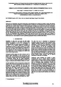
Visual interpretation based on knowledge acquired during field studies reveals an overrepresentation of Sycamore maple (AP), European ash (FS), European larch (LD), and European silver fir (AA) in the classification maps. This can also be seen in Figure 10 which shows the percentage of classified tree species derived from the classification maps. The labelled percentages show the percentage of tree species in the upper layer based on the forest inventory results of the entire BFNP area. An important consideration with respect to the classification results displayed in Figure 10 is that the classified maps only cover about 65% of the total national park area.

Figure 10: Percentage of classified tree species compared to the results of the forest inventory. Labelled percentages show the forest inventory results of tree species in the upper layer.

EARSeL eProceedings 14, Special Issue 2, 2015-16: 9th EARSeL Imaging Spectroscopy Workshop, 2015

65

Based on visual interpretation of the resulting maps, it can be seen that areas of the BFNP actually covered by Norway spruce or European beech show misclassification patterns in the maps caused by topographic features included in the classification model. This means that Norway spruce stands located in small valleys or lower elevations tend to be classified as tree species only occurring in these lower elevation zones such as Scots pine, Douglas fir or European silver fir. The same behaviour can be observed for European beech stands located in lower elevations which are classified as European alder or European white birch. The classification maps are also influenced by remaining BRDF effects in the overlap areas of the flight lines which in turn influenced the calculated vegetation index maps included in the classification. These effects cause sudden changes of homogeneous beech stands to tree species like European ash or sycamore maple, indicating a high similarity between these tree species. Such patterns are also visible in homogeneous Norway spruce stands which show abrupt changes to European larch or European silver fir. From a visual point of view, the tree species classification is strongly influenced by the relief of the BFNP. DISCUSSION AND CONCLUSIONS

The aim of this study was to develop a multi-source approach for tree species classification adapted to the needs of the BFNP. The study focused on the suitability of tree species features derived from hyperspectral signatures and LiDAR data. For testing the potential of a multi-source classification approach in forest mapping, a reference data set from 13 tree species was created. The retrieved spectral, structural, and topographic features were analysed with the Random Forest classifier. The final analysis revealed successful discrimination of tree species with an overall accuracy of 94%. However, care must be taken when using elevation as one parameter for the classification. As mentioned before, misclassification patterns occurred in the final tree species maps based on the relief of the study area. Therefore, it is important that the training and test data set covers all possible terrain-specific variations of the occurring tree species. This means that reference data must consider spatial signatures and the training and test sites must - if possible - be evenly distributed over the whole study area. Due to the limited accessibility of big areas in the National Park, the in situ data collection for this analysis mainly focussed on the lower elevations of the southern part, i.e. the Rachel-Lusen region. This may have led to misclassification especially in the northern image. A classification based on training data acquired in the southern part may not be able to reproduce the forest structure of the northern part of the BFNP, i.e. the Falkenstein-Rachel region, which is still strongly characterized by forest management in contrast to the Rachel-Lusen region (13). In general, predictive classification models trained with a small number of samples to a large complex forest area, such as the BFNP, are error-prone, because the samples usually do not cover the spatial, spectral, structural and topographic variability of the forest. Due to the described heterogeneous stand structure it was quite difficult to find enough specimens especially of rare tree species such as Douglas fir and Scots pine. Adult full-grown specimens of pioneer tree species such as European white birch or European rowan with large crowns providing enough training pixels for model creation were rare. For this reason, an iterative expansion of field data is recommended to improve mapping of tree species. This means that ground based verification of the classified trees could be used to gather more suitable reference data to represent the full range of conditions present at the BFNP. Random Forest proved to be useful for species discrimination based on a large feature database. Applying RF to a stratified randomly sampled training set led to very high model and classification accuracies. Confusion between European larch and Norway spruce indicates a strong similarity of these two species regarding spectral, structural, and topographic features. This confusion led to an over-representation of European larch in the classification maps. Lowest classification accuracies were found for European white birch, Scots pine and European rowan. It was difficult to find reliable reference samples for these tree species, as they usually do not occur in pure stands in the

EARSeL eProceedings 14, Special Issue 2, 2015-16: 9th EARSeL Imaging Spectroscopy Workshop, 2015

66

BFNP. Therefore, some misclassifications may result from the low number of available reference data and possible errors in the reference data set resulting from potentially included background reflectance and mixed or shadowed pixels. A future step will be to examine the inclusion of a shadow mask in order to overcome the aforementioned problems. Also an object-based classification using the tree crowns delineated from the LiDAR data could be an alternative approach. Regarding accuracy assessment, the OOB validation technique provided by RF must be used with caution. OOB validation performed on training data may be biased which usually leads to higher classification accuracies than a validation based on an independent test data set. Therefore, it is important to provide a large number of test pixels, which were unfortunately not available for this study. The evidence from this study is that the data sets used for the RF model produced reliable and accurate species distribution maps for 13 tree species in some parts of the BFNP, which will be valuable for assisting management. There are problems in the lower elevations of the national park caused by topographic features included in the classification model. These tree species distribution maps can then be implemented in future ecological studies conducted in the study area. However, it is important to consider the complexity of forest environments and their interactions with many ecological factors that need to be addressed for tree species mapping, including habitat types, plant communities, landforms, soil composition and disturbance history (52,53). Incorporating these factors into the classification model could result in more accurate maps which can help to understand the ecological processes and effects of environmental factors on species distribution and density (e.g. bark beetle impacts on Norway spruce). To improve tree species classification, additional information from the SWIR region of the spectrum could be used. Several vegetation biochemicals, such as lignin and cellulose, create absorption features across the SWIR region. By using data from the HySpex SWIR sensor, additional spectral bands are available and more vegetation indices can be calculated, which can provide better information about phenology, structure and biochemistry of the various tree species (54,31). Several studies also recommended multi-seasonal classification approaches using data acquired at different phenological stages (7,55,56). Considerable differences in spectral reflectance occur with the aging of leaves due to growth processes and changes in leaf pigments. Knowledge of the leaf ontogeny by species and season is helpful in image analysis, in order to highlight differences between tree species (53). The spectral data used in this study was acquired in July when phenological activity of tree species is usually low (57). This leads to very similar spectral responses from the different tree species. Multi-seasonal hyperspectral data may therefore enhance tree species classification results. ACKNOWLEDGEMENTS

This work is based on the ideas of the newly established Data Pool Forestry, which is an international collaboration for the purpose of making in situ and remotely sensed data available to foster international research cooperation. The Data Pool Initiative for the Bohemian Forest Ecosystem consists of seven parties, involving among others the Bavarian Forest National Park, the Czech Šumava National Park and the German Aerospace Center (DLR). The authors would like to thank two anonymous reviewers for valuable comments and helpful suggestions. REFERENCES

1

Reitberger J, P Krzystek & M Heurich, 2006. Full-waveform analysis of small footprint airborne laser scanning data in the Bavarian Forest National Park for tree species classification, pp.

EARSeL eProceedings 14, Special Issue 2, 2015-16: 9th EARSeL Imaging Spectroscopy Workshop, 2015

67

229-238. Workshop on 3D Remote Sensing in Forestry (Vienna, Austria) 401 pp. (last date accessed: 22.01.2016) 2

Latifi H, F E Fassnacht, J Müller, A Tharani, S Dech & M Heurich, 2015. Forest inventories by LiDAR data: a comparison of single tree segmentation and metric-based methods for inventories of a heterogeneous temperate forest. International Journal of Applied Earth Observation and Geoinformation, 42: 162-174

3

Clark M L & D A Roberts, 2012. Species-level differences in hyperspectral metrics among tropical rainforest trees as determined by a tree-based classifier. Remote Sensing, 4(12): 1820-1855

4

Dalponte M, H O Orka, T Gobakken, D Gianelle & E Naesset, 2013. Tree species classification in boreal forests with hyperspectral data. IEEE Transactions on Geoscience and Remote Sensing, 51(5): 2632-2645

5

Dalponte M, L Bruzzone & D Gianelle, 2012. Tree species classification in the Southern Alps based on the fusion of very high geometrical resolution multispectral/hyperspectral images and LiDAR data. Remote Sensing of Environment, 123: 258-270

6

Jones T G, N C Coops & T Sharma, 2010. Assessing the utility of airborne hyperspectral and LiDAR data for species distribution mapping in the coastal Pacific Northwest, Canada. Remote Sensing of Environment, 114(12): 2841-2852

7

Cho M A, R Mathieu, G P Asner, L Naidoo, J van Aardt, A Ramoelo, P Debba, K Wessels, R Main, I P J Smit & B Erasmus, 2012. Mapping tree species composition in South African savannas using an integrated airborne spectral and LiDAR system. Remote Sensing of Environment, 125: 214-226

8

Franklin S E, 1994. Discrimination of subalpine forest species and canopy density using digital CASI, SPOT PLA, and Landsat TM data. Photogrammetric Engineering & Remote Sensing, 60(10): 1233-1241

9

Higgins M A, G P Asner, R E Martin, D E Knapp, C Anderson, T Kennedy-Bowdoin, R Saenz, A Aguilar & S Joseph Wright, 2014. Linking imaging spectroscopy and LiDAR with floristic composition and forest structure in Panama. Remote Sensing of Environment, 154: 358-367

10 Yao W, P Krzystek & M Heurich, 2012. Tree species classification and estimation of stem volume and DBH based on single tree extraction by exploiting airborne full-waveform LiDAR data. Remote Sensing of Environment, 123: 368-380 11 Ghosh A, F E Fassnacht, P K Joshi & B Koch, 2014. A framework for mapping tree species combining hyperspectral and LiDAR data: Role of selected classifiers and sensor across three spatial scales. International Journal of Applied Earth Observation and Geoinformation, 26: 4963 12 Kiener H, M Hußlein & K H Englmaier, 2008. Natura 2000 - Management im Nationalpark Bayerischer Wald. Nationalparkverwaltung Bayerischer Wald, Wissenschaftliche Schriftenreihe Heft 17, 252 pp. 13 Heurich M, B Beudert, H Rall & Z Křenová, 2010. National Parks as model regions for interdisciplinary long-term ecological research: The Bavarian Forest and Šumavá National Parks underway to transboundary ecosystem research. In: Long-term Ecological Research. Between Theory and Application, Müller F, C Baessler, H Schubert & S Klotz (Editors), 456 pp. (Springer, Netherlands) 327-344 14 Heurich M & K H Englmaier, 2010. The development of tree species composition in the Rachel-Lusen region of the Bavarian Forest National Park. Silva Gabreta, 16(3): 165-186

EARSeL eProceedings 14, Special Issue 2, 2015-16: 9th EARSeL Imaging Spectroscopy Workshop, 2015

68

15 Lausch A, M Heurich & L Fahse, 2013. Spatio-temporal infestation patterns of Ips typographus (L.) in the Bavarian Forest National Park, Germany. Ecological Indicators, 31: 73-81 16 Heurich M & M Neufanger, 2005. Die Wälder des Nationalparks Bayerischer Wald. Ergebnisse der Waldinventur 2002/2003 im geschichtlichen und waldökologischen Kontext. Nationalparkverwaltung Bayerischer Wald, Wissenschaftliche Schriftenreihe Heft 16, 178 pp. 17 Habermeyer M, A Müller, S Holzwarth, R Richter, R Müller, M Bachmann, K-H Seitz, P Seifert & P Strobl, 2005. Implementation of the automatic processing chain for ARES. In: Zagajewski B, M Sobczak & M Wrzesien (Editors) 4th EARSeL Workshop on Imaging Spectroscopy, 6775 18 Richter R & D Schläpfer, 2015. Atmospheric / Topographic Correction for Airborne Imagery. DLR/ReSe Applications, Wessling, DLR-IB 565-02/15, Version 7.0.1, 252 pp. (last date accessed: 8 January 2016) 19 Müller R, M Lehner, R Müller, P Reinartz, M Schroeder & B Vollmer, 2002, A program for direct georeferencing of airborne and spaceborne line scanner images. ISPRS Archives, XXXIV(1), 6 pp. 20 Schläpfer D, R Richter & T Feingersh, 2015. Operational BRDF effects correction for WideField-of-View Optical Scanners (BREFCOR). IEEE Transactions on Geoscience and Remote Sensing, 53(4), 1855-1864 21 Rogge D M & B Rivard, 2010. Iterative spatial filtering for reducing intra-class spectral variability and noise. 2nd Workshop on Hyperspectral Image and Signal Processing: Evolution in Remote Sensing (WHISPERS) 575 pp. IEEE Catalog Number: CFP 1048H-PRT, 142-145 22 Heurich M, F Fischer, O Knörzer & P Krzystek, 2008. Assessment of digital terrain models (DTM) from data gathered with airborne laserscanning in temperate European beech (Fagus sylvatica) and Norway spruce (Picea abies) forests. Photogrammetrie, Fernerkundung, Geoinformation, 6: 473-488 23 Asner G P, D E Knapp, T Kennedy-Bowdoin, M O Jones, R E Martin, J Boardman & R F Hughes, 2008. Invasive species detection in Hawaiian rainforests using airborne imaging spectroscopy and LiDAR. Remote Sensing of Environment, 112(5): 1942-1955 24 Weier J & D Herring, 2000. Measuring Vegetation (NDVI & EVI). NASA Earth Observatory (last date accessed: 13.03.2015) 25 Roloff A, H Weisgerber, U Lang & B Stimm, 2010. Bäume Mitteleuropas (Wiley-VCH, Weinheim, Germany) 480 pp. 26 Bajwa S G, P Bajcsy, P Groves & L F Tian, 2004. Hyperspectral image data mining for band selection in agricultural applications. Transactions of the American Society of Agricultural Engineers, 47(3): 895-908 27 Wu C, 2004. Normalized spectral mixture analysis for monitoring urban composition using ETM+ imagery. Remote Sensing of Environment, 93(4): 480-492 28 Clark M L & D A Roberts, 2012. Species-level differences in hyperspectral metrics among tropical rainforest trees as determined by a tree-based classifier. Remote Sensing, 4(12): 1820-1855 29 Jordan C, 1969. Leaf-area index from quality of light on the forest floor. Ecology, 50(4): 663666

EARSeL eProceedings 14, Special Issue 2, 2015-16: 9th EARSeL Imaging Spectroscopy Workshop, 2015

69

30 Gitelson A & M Merzlyak, 1994. Spectral reflectance changes associated with autumn senescence of Aesculus Hippocastanum L. and Acer Platanoides L. leaves. Journal of Plant Physiology, 143: 286-292 31 Roberts D A, K L Roth & R L Perroy, 2012, Hyperspectral Vegetation Indices. In P. S. Thenkabail, J. G. Lyon and A. Huete (Editors), Hyperspectral Remote Sensing of Vegetation, 782 pp. (CRC Press Taylor & Francis Group, Boca Raton, FL, USA) 309-327 32 Horler D, M Dockray & J Barber, 1983. The red edge of plant leaf reflectance. International Journal of Remote Sensing, 4, 273-288 33 Pu R, P Gong, G S Biging & M R Larrieu, 2003. Extraction of red edge optical parameters from hyperion data for estimation of forest leaf area index. IEEE Transactions on Geoscience and Remote Sensing, 41(4): 916-921 34 Treitz P M & P J Howarth, 1999. Hyperspectral remote sensing for estimating biophysical parameters of forest ecosystems. Progress in Physical Geography, 23(3): 359-390 35 Gamon J, L Serrano & J Surfus, 1997. The photochemical reflectance index: An optical indicator of photosynthetic radiation-use efficiency across species, functional types, and nutrient levels, Oecologia, 112: 492-501 36 Naidoo L, M Cho, R Mathieu & G Asner, 2012. Classification of savanna tree species, in the Greater Kruger National Park region, by integrating hyperspectral and LiDAR data in a Random Forest data mining environment. ISPRS Journal of Photogrammetry and Remote Sensing, 69: 167-179 37 Wood J, 1996. The Geomorphological Characterization of Digital Elevation Models. Ph.D. Thesis, Department of Geography, University of Leicester, UK 38 Dalponte M, H O Ørka, L T Ene, T Gobakken & E Næsset, 2014. Tree crown delineation and tree species classification in boreal forests using hyperspectral and ALS data. Remote Sensing of Environment, 140: 306-317 39 Breiman L & A Cutler, 2004. Random Forests (last date accessed: 22.02.2015) 40 Cutler D R, T C Edwards, K H Beard, A Cutler, K T Hess, J Gibson & J J Lawler, 2007. Random forests for classification in ecology. Ecology, 88(11): 2783-2792 41 Pal M, 2005. Random forest classifier for remote sensing classification. International Journal of Remote Sensing, 26(1): 217-222 42 Jensen J R, 2005. Introductory Digital Image Processing, 3rd Edition (Prentice-Hall Series in Geographic Information Science. Pearson Education, Inc., Upper Saddle River, NJ.) 526 pp. 43 Richards J A & X Jia, 2005. Remote Sensing Digital Image Analysis: An Introduction, 4th Edition (Springer, New York, USA) 464 pp. 44 Chen C, A Liaw & L Breiman, 2004. Using Random Forest to Learn Imbalanced Data (University of California, Berkeley, USA) 12 pp. (last date accessed: 22.01.2016) 45 Roberts D A, S L Ustin, S Ogunjemiyo, J Greenberg, S Z Dobrowski, J Chen &T M Hinckley, 2004. Spectral and structural measures of northwest forest vegetation at leaf to landscape scales. Ecosystems, 7: 545-562 46 Rautiainen M, P Stenberg, T Nilson & A Kuusk, 2004. The effect of crown shape on the reflectance of coniferous stands. Remote Sensing of Environment, 89: 41-52 47 Guyot G, F Baret & D Major, 1988. High spectral resolution: Determination of spectral shifts between the red and infrared. ISPRS Archives, XXVII(B7): 750-760

EARSeL eProceedings 14, Special Issue 2, 2015-16: 9th EARSeL Imaging Spectroscopy Workshop, 2015

70

48 Thenkabail P S, J G Lyon & A Huete, 2012. Advances in hyperspectral remote sensing of vegetation and agricultural croplands. In: Thenkabail P S, J G Lyon & A Huete (Editors), Hyperspectral Remote Sensing of Vegetation, 782 pp. (CRC Press, Boca Raton, FL, USA) pp. 335 49 Liaw A & M Wiener, 2002. Classification and regression by randomForest. R News, 2(3): 18-22 50 Lillesand T M, R W Kiefer & J W Chipman, 2008. Remote Sensing and Image Interpretation, 6th Edition (John Wiley & Sons) 768 pp. 51 Foody G, 2002. Status of land cover classification accuracy assessment. Remote Sensing of Environment, 80: 185-201 52 Clark M L, D A Roberts & D B Clark, 2005. Hyperspectral discrimination of tropical rain forest tree species at leaf to crown scales. Remote Sensing of Environment, 96: 375-398 53 Howard J A, 1991. Remote Sensing of Forest Resources. 1st Edition (Chapman & Hall, London, UK) 420 pp. 54 Lucas R, P Bunting, M Paterson & L Chisholm, 2008. Classification of Australian forest communities using aerial photography, CASI and HyMap data. Remote Sensing of Environment, 112(5): 2088-–2103 55 Elatawneh A, A Rappl, N Rehush, T Schneider & T Knoke, 2013. Forest tree species communities identification using multi phenological stages RapidEye data: Case study in the forest of Freising. In: 5. RESA Workshop, pp. 21-39 56 Krahwinkler P M & J Rossmann, 2010. Analysis of hyperspectral and high-resolution data for tree species classification. ASPRS 2010 Annual Conference, 9 pp. 57 DWD Climate Data Center, 2015. Phenological data reported by annual reporters. CDC ftpserver (last date accessed: 26.03.2015)