Feedforward joint phase and timing estimation with ... - IEEE Xplore

824

IEEE TRANSACTIONS ON VEHICULAR TECHNOLOGY, VOL. 48, NO. 3, MAY 1999

Feedforward Joint Phase and Timing Estimation with OQPSK Modulation Antonio A. D’Amico, Aldo N. D’Andrea, Senior Member, IEEE, and Umberto Mengali, Fellow, IEEE

Abstract—We propose an algorithm for joint carrier phase and timing estimation with offset quadriphase modulation (OQPSK) signaling. The derivation is based on maximum-likelihood arguments and leads to a feedforward structure that operates on signal samples taken at bit rate. Phase and timing algorithms operate in parallel—not sequentially—and provide their estimates in a fixed time. The synchronizer is readily implemented in digital form and is particularly suitable for burst mode transmissions. Its performance is analytically assessed and verified by simulations. Comparisons are made with other methods described in the literature. Index Terms— Digital communications, offset quadriphase modulation, synchronization.

I. INTRODUCTION

O

FFSET quadriphase modulation (OQPSK) is a signaling scheme similar to conventional QPSK, except that the bit transitions on the sine and cosine carriers are offset in s, the inverse of the bit rate. With bandlimited time by signaling, this results in a maximum envelope variation of only 3 dB (70%), as opposed to 100% with QPSK. Limited envelope variations are necessary to control adjacent channel interference in microwave radio systems employing power-efficient amplifiers. With filtered QPSK, the amplifier nonlinearity causes a significant regeneration of the signal spectrum back to the unfiltered level. By contrast, fairly limited sidelobe restoration occurs with OQPSK [1], [2]. Superficially, OQPSK and QPSK receivers have similar between the structures, apart from the obvious delay by regenerated data stream on the quadrature rail. As is now explained, however, some important differences related to the synchronization functions exist that make the design of OQPSK modems comparatively difficult. The crucial point is that all of the OQPSK timing algorithms known today are carrier-phase sensitive and have poor performance for certain phase errors [3]. This is in contrast with QPSK modulation for which various phase-insensitive timing recovery schemes are available with excellent performance [4], [5]. In an OQPSK receiver, the phase sensitivity causes long acquisitions due to complex interactions between phase and timing loops. Long acquisitions are only tolerable with continuous signaling. In burst mode transmissions, they entail information rate reductions and should be avoided.

Manuscript received October 1996; revised July and November 1997. The authors are with the Department of Information Engineering, Universit`a di Pisa, 56100 Pisa, Italy. Publisher Item Identifier S 0018-9545(99)01035-X.

In this paper, we investigate joint phase and timing estimation in OQPSK using maximum-likelihood (ML) arguments. As we shall see, this approach leads to a feedforward estimation scheme wherein phase and timing are separately measured from asynchronous signal samples. In other words, the timing estimator is phase insensitive and the phase estimator operates in a clockless fashion. The overall scheme is easily implemented in digital form and is appealing for applications where short acquisitions are required. The paper is organized as follows. In the next section, we derive an approximate expression of the likelihood function for carrier phase and timing. In Section III, this function is maximized and the location of the maximum is used as an estimator for the unknown synchronization parameters. Performance analysis is carried out in Section IV while simulation results are discussed in Section V. Conclusions are drawn in Section VI. II. APPROXIMATE LIKELIHOOD FUNCTION The received baseband waveform is the sum of signal plus noise. The noise component is modeled as a complex-valued white Gaussian process with independent real and imaginary . The parts, each with two-sided power spectral density signal component has the form

(1) is where is the carrier phase, is the timing epoch, and a real-valued signaling pulse, and represent the data symbols on the in-phase and quadrature rails. They are independent, identically distributed, and take on the values 1 with equal probability. and are all unknown at the receiver Parameters and must be estimated. In this study, we consider a twoare estimated first and their step procedure wherein values are exploited for data detection. The second step is straightforward, however, and is not covered in the sequel. Only the estimation of and is addressed. To this end the following discrete-time approach is adopted. The received waveform is first passed through an antialiasing , a multiple filter (AAF) and then is sampled at some rate of Although an oversampling factor of two is adequate in many practical cases, the ensuing formulas are developed for

0018–9545/99$10.00  1999 IEEE

D’AMICO et al.: FEEDFORWARD JOINT PHASE AND TIMING ESTIMATION

a generic Also, the assumption is made that: 1) the AAF has sufficiently large not to distort the signal a bandwidth ; and 3) the components; 2) the sampling rate equals noise samples are independent (which occurs, in particular, if the AAF transfer function is rectangular, but other more practical filter transfer functions are conceivable). In these from the AAF contain the conditions, the samples same information as the incoming waveform and the problem from the observation of arises of estimating the pair consecutive samples. Note that represents the length of the observation interval. This problem can be pursued making use of maximum likelihood (ML) arguments. In particular, in this section we derive an (approximate) expression of the likelihood function for the parameters and , and then (in the next section) we compute the location where the function achieves a maximum. This will provide us with an (approximate) ML estimate of . the As a first step in this direction denote by samples from the AAF, with indexes from zero to Then, the ML function for the signal parameters takes on the form [6, ch. 3]

825

with no guarantee of useful results. So, rather than taking a fruitless avenue, we follow a modest path which has the merit of leading to a closed-form solution. It is worth adding that this quadratic approximation is very popular in the literature and has been adopted in similar circumstances [8], [9] in view of its analytical tractability. To proceed further, we write the first sum in (2) as (4) with (5) (6)

(7) Then, expanding the exponential in (2) and neglecting immaterial constants leads to (8)

(2)

over and is At this point, the average of readily computed. In particular, in Appendix A it is shown that (9)

where while

can be put in the form

(10)

(3) where the following notations have been used: and notations of the type are used to indicate “trial value of .” Note that there are four distinct parameters in the above and As we mentioned earlier, however, equations: we are only interested in the first two: and Following [6], we can dispose of the others by concentrating on the function , the average of over and . proves Unfortunately, a rigorous calculation of to be intractable and we are forced to make two major approximations. The first one involves dropping the second summation in (2). In principle, this would be allowed only if the sum were independent of all the unknown parameters. On and but people often the contrary, the sum depends on argue that the dependence is weak and can be neglected. Here, we shall follow this trend although we expect that it will result in the generation of self-noise [7]. The second approximation relies on the assumption that the signal-to-noise ratio (SNR) is so low that the exponential in (2) can be replaced by its Taylor series truncated to the quadratic term. This means that the truncation will be valid only at very low SNR’s, probably lower than the SNR’s of practical interest. On the other hand, the addition of further terms in the series would enormously complicate the analysis

(11)

(12)

(13)

(14) (15) In the above equations, the function transform

has the Fourier (16)

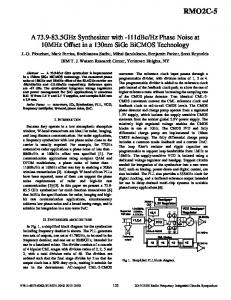
is the Fourier transform of From (16) and the and (which holds because is real property is even. Fig. 1 illustrates the valued) it can be shown that

826

IEEE TRANSACTIONS ON VEHICULAR TECHNOLOGY, VOL. 48, NO. 3, MAY 1999

which indicates that the maxima occur only when and are even numbers, say equal to and In other words, the locations for the maxima are expressed by (23) (24) for arbitrary integers and The following remarks are of interest. 1) From (24) it appears that the timing estimates are am. This should be expected in biguous by multiples of delay between I and Q signal components. view of 2) For a given timing estimate (i.e., for a fixed ), (23) says that the phase estimates are ambiguous by multiples of . Again, this is intuitively obvious since (1) may also be written as

(25) Fig. 1. Function q (t) for some rolloff values.

shape of for a root-raised-cosine rolloff function with rolloff It is clear from (11) and (12) that and are both independent of and In Appendix A, it is proved that this is also true for the sum in (15). Putting all these facts together and pruning off further immaterial constants, it is concluded that the expectation of (8) over and may be rewritten as (17) In the next section, we exploit this result to estimate III. JOINT PHASE

AND

and

TIMING ESTIMATOR

To locate the maximum of derivatives

we consider the partial

(18)

or may which says that either be viewed as the unknown signal parameters. 3) As differential encoding/decoding can be used to resolve the above ambiguities [10, ch. 4], in the sequel we for simplicity. arbitrarily set The above estimation algorithm is now simplified by writing and in (11) and (12) in a more convenient form. The has a duration procedure involves three steps. First, since of few symbol intervals around the origin (see Fig. 1) and the estimation interval comprises in general many symbols , (13) and (14) are only marginally affected if to In this way the summations are extended from and may be regarded as outputs of two (nonand , driven by causal) filters, and , respectively. Second, the filters can be made causal by shifting their samples. The shift must impulse responses rightward by be sufficiently large to make the tails of the impulse responses on the negative axis negligible. As a result the filter outputs steps and become are delayed by (26)

(19) Setting them to zero and solving for

and

(27)

yields (20)

and Third, inserting and (12) and suitably delaying and expressions of

into (11) produces the desired

(21) and are integers such is even and the where and are restricted to the interval . arguments of do not all correspond It should be noted that the pairs In fact, inserting (20) and (21) into to maxima for (17) and rearranging produces (22)

(28)

(29)

D’AMICO et al.: FEEDFORWARD JOINT PHASE AND TIMING ESTIMATION

827

Fig. 2. Block diagram of the estimator.

A block diagram of the joint phase and timing estimator is illustrated in Fig. 2. Some observations can be made about is real valued, it follows this scheme. First, when This implies from (16) that which means that the filters are real. Second, a considerable equals simplification occurs when the oversampling factor two, as occurs with rolloff values less than unity. In these and reduce circumstances the exponentials and , respectively, and the multiplications to involve only sign inversions and/or exchanges by . Thus, significant between real and imaginary parts of savings in computational load are possible. Third, it should be stressed that phase and timing are estimated in parallel, not sequentially. This implies that the phase estimator does not need any timing information.

referred to as self-noise and represents the residual variance when grows large. and depend on various In general system parameters as, for example, the oversampling factor, the shape of the signaling pulse, the length of the observaTo be specific, we provide tion interval, and the delay approximate formulas and graphs for these coefficients under the following simplifying assumptions. is a root-raised-cosine 1) The Fourier transform of rolloff function. 2) The frequency response of the AAF is rectangular of . bandwidth 3) The oversampling factor equals two. is much larger than 4) The observation interval (32)

IV. ANALYSIS The performance of the above estimator can be conveniently expressed in terms of mean and variance of the estimates. Calculations of these statistics are developed in [11] along the lines described in [5] and [6, ch. 9]. Unfortunately, the passages are very cumbersome and cannot be reported here. Only the final results are given. It turns out that both phase and timing estimator are unbiased. Also, the normalized timing variance (normalization is ) has the form performed with respect to

(30) A similar expression applies to the phase error variance (in rad )

(31) is the SNR and the coefficients In these formulas, , and reflect interactions Signal Signal, Signal Noise, and Noise Noise taking place in is the estimation process. In particular, the ratio

In these conditions, the coefficients the simple expressions

and

have

(33) (34) and , they depend on the length of As for the observation interval and the rolloff factor as indicated in Figs. 3 and 4. Two remarks about these results are useful. First, the coand also depend on However, the efficients dependence is weak and can be ignored for practical purposes (Figs. 3 and 4 have been drawn for and equal to zero). Second, it is clear from (33) and (34) and the graphs in Figs. 3 and 4 that the estimation accuracy worsens as the rolloff decreases. Thus, the proposed synchronization method is unsatisfactory for signals with little excess bandwidth and fails completely with zero excess bandwidth. This drawback is also encountered with nondata-aided (NDA) estimation schemes suitable for nonoffset modulations [3]–[5]. V. SIMULATION RESULTS AND COMPARISONS Simulations have been run to verify the theory in the previous section and to compare the performance of the proposed synchronizer with other methods discussed in the

828

IEEE TRANSACTIONS ON VEHICULAR TECHNOLOGY, VOL. 48, NO. 3, MAY 1999

(

SS ) versus observation length L . 0

Fig. 3. Coefficients KT

Fig. 5. Phase error variance versus Es =N0 with rolloff as a parameter.

a root-raised-cosine rolloff and the parameter has been set equal to 100. Figs. 5 and 6 illustrate phase and timing estimation variances. Continuous lines represent the theory as given by (30) and (31) while the straight lines indicate lower bounds for the phase and timing estimation. They are approximate Cramer–Rao bounds and are derived in Appendix B assuming optimistically known transmitted symbols and a long observation interval . As these bounds coincide with the modified Cramer–Rao bounds discussed in [12], in the following they are denoted by the acronym MCRB. They are expressed by MCRB

(35)

MCRB

(36)

with (37)

SS ) versus observation length L . 0

(

Fig. 4. Coefficients KP

literature. The antialiasing filter has been modeled as an eightpole Butterworth finite impulse response (FIR) type with a . An oversampling factor of two has 3-dB bandwidth of been adopted. Different values for the delay have been used, has been depending on the rolloff factor. In particular, , with , and with chosen with . Finally, has been given a Fourier transform with

is a function of the rolloff and decreases Note that MCRB is shown as increases. However, only the bound with in Fig. 6 so as not to cram the picture. As is seen, theory and simulations agree well, apart from some minor inconsistencies at low rolloff values. They arise from the fact that assumption and (as used (32) is not well satisfied for ). Further results (not shown) indicate that the with inconsistencies disappear for longer observation intervals. It is interesting to compare the performance of the present estimator with that of other schemes suitable for either OQPSK or QPSK. Let us first concentrate on phase estimation. A natural reference is the NDA algorithm proposed by Asheid

D’AMICO et al.: FEEDFORWARD JOINT PHASE AND TIMING ESTIMATION

Fig. 6. Timing error variance versus

Es =N0 with rolloff as a parameter.

and Moeneclaey (A&M) in [13] for OQPSK. As is known, this algorithm operates on the samples and derived from the matched from filter. Note that the samples are taken at multiples of , which implies that clock information must be available. The samples are first fed to a nonlinear circuit that performs the transformation (38) is some suitable function of ( is estimated as

) and then the phase

829

Fig. 7. Phase error variance with A&M estimator. Dashed lines correspond to the results in Fig. 5 for  = 0:25 and  = 0:5.

which, however, is only applicable to QPSK, not OQPSK. The O&M algorithm is expressed by (40) are samples from the matched filter taken at where [which means in (40)]. Fig. 8 illustrates a rate simulations with the O&M algorithm. Dashed lines represent and . It is seen that the results in Fig. 6 for the estimation variance with O&M is nearly the same as with the proposed algorithm at SNR values of practical interest. VI. CONCLUSIONS

(39) The performance of (39) is assessed in [6] by simulation . It turns out that the choice of for different functions has marginal consequences with rolloff factors greater is almost than 0.5. For smaller values, the option optimum. Fig. 7 illustrates simulations obtained in this case. The dashed lines represents the results in Fig. 5 for and . It is seen that A&M has virtually the same at SNR performance as the proposed method for , the A&M algorithm values of practical interest. For is somewhat superior. Turning to timing estimation, we cannot compare our synchronizer with others suitable for OQPSK since all the existent methods are phase dependent. The only scheme that comes to mind is that proposed by Oerder and Meyr (O&M) in [5]

A joint phase and timing estimator for OQPSK modulation has been derived making use of ML-oriented arguments. The estimator has a feedforward structure and operates on . Timing asynchronous signal samples taken at a rate and phase algorithms work in parallel, not sequentially, and provide their estimates in a fixed time. They can readily be implemented in digital form and are suited for burst mode transmission. Analytical formulas and graphs have been provided to compute phase and timing error variances as a function of various system parameters like the excess bandwidth factor, the observation length and the SNR. The theoretical results agree well with the simulations. It turns out that the proposed method has very good performance except with very small rolloff factors. Comparisons have been made with other phase and timing synchronizers. In particular, the phase synchronizer accuracy has been compared with that of the clock-aided method

830

IEEE TRANSACTIONS ON VEHICULAR TECHNOLOGY, VOL. 48, NO. 3, MAY 1999

Next, writing

and

in the form (A.5) (A.6)

and substituting into (A.4) yields

(A.7) with (A.8) Assuming is independent of

for , we now show that and the sum in (A.7) may be written as (A.9)

where

(A.10) Fig. 8. Timing error variance with O&M estimator. Dashed lines correspond to the results in Fig. 6 for  = 0:25 and  = 0:5.

(A.11)

by Asheid and Moeneclaey. The results are similar for excess bandwidth factors of 0.5 or greater. The Asheid and Moeneclaey method is somewhat superior with smaller rolloffs.

(A.12) The proof relies on the following version of the Poisson sum formula:

APPENDIX A In this Appendix, we compute the expectation of and over and . We begin with the definition of

(A.13) (A.1) where

and are arbitrary functions and are their Fourier transforms. Let us first concentrate on . Inserting (A.2) into (A.8) yields

where

(A.2) As the data have zero mean, it follows from (A.1) that (A.3) . From (A.1) and the Next, we concentrate on and (recall that they are statistics of the sequences independent and each consists of independent and zero-mean symbols), it is readily shown that

(A.14) On the other hand, application of (A.13) for and bandlimited to produces

(A.15)

(A.4) from which it follows that

is independent of .

D’AMICO et al.: FEEDFORWARD JOINT PHASE AND TIMING ESTIMATION

831

Thus, substituting (B.1) and (B.2) into (B.4)–(B.6) and bearing in mind that

Next, we turn to (A.9). From (A.2), we obtain

(B.7) after some manipulations we obtain

(A.16) On the other hand (B.8)

(A.17) Application of (A.13) to each sum in the right-hand side of (A.17) leads eventually to (A.9).

(B.9)

APPENDIX B In this Appendix, we compute the Cramer–Rao bounds for the estimation variances of the phase and timing parameters. Our discussion begins with the likelihood function for and , i.e.,

(B.10) (B.1) with

(B.2) It should be noted that (B.1) and (B.2) have essentially the same form as (2) and (3) in the text, except that the data symbols here bear no tilde as they are no longer viewed as random variables, but (optimistically) as known quantities. The Fisher information matrix for and takes the form [6] (B.3) with (B.4)

(B.5)

is the derivative of where As expected, the elements of are functions of and , which means that there are many different matrix values depending on the symbol sequences. As the Cramer–Rao bounds (CRB’s) are the diagonal elements of , it follows that these bounds depend on the inverse of and we consider. the particular pair of sequences This is a rather uncomfortable situation as, in many practical and are random and there is no specific cases, realization of theirs which can be taken as a reference. A and as way out of this difficulty is to think of the outputs of two separate data generators, each providing a stream of independent and equally likely symbols 1. Under these conditions we expect from the ergodic theorem that, as the length of the observation interval grows large, the summations in (B.8)–(B.10) ultimately approach their ensemble averages and the Fisher information matrix becomes and . In the following, we pursue independent of this approach which is approximate since, in practice, the parameter may not be long enough to justify the procedure. Taking the ensemble averages of (B.8)–(B.10) and rearranging yields

(B.6) where the expectations are computed over the noise process.

(B.11)

832

IEEE TRANSACTIONS ON VEHICULAR TECHNOLOGY, VOL. 48, NO. 3, MAY 1999

(B.12)

(B.13) Next, denoting by

the Fourier transform of (B.14)

and using the Poisson sum formula we get (B.15) is This equation takes a particularly simple form if and is less than or equal to bandlimited to (which means an oversampling factor ). Under these conditions we get

(B.16) With similar arguments, it can be shown that

[6] S. M. Kay, Fundamentals of Statistical Signal Processing. Englewood Cliffs, NJ: Prentice-Hall, 1993. [7] M. H. Meyrs and L. E. Franks, “Joint carrier phase and symbol timing for PAM systems,” IEEE Trans. Commun., vol. COM-28, pp. 1121–1129, Aug. 1980. [8] M. Moeneclaey and G. de Jonghe, “Tracking performance comparison of two ML-oriented carrier-independent NDA symbol synchronizers,” IEEE Trans. Commun., vol. 40, pp. 1423–1425, Sept. 1992. [9] K. Goethals and M. Moeneclaey, “Tracking performance of ML-oriented NDA symbol synchronizers for nonselective fading channels,” IEEE Trans. Commun., vol. 43, pp. 1179–1184, Feb./Mar./Apr. 1995. [10] K. Feher, Digital Communications. Englewood Cliffs, NJ: PrenticeHall, 1981. [11] A. D’Amico, “Synchronization issues with OQPSK and CPM transmissions,” Internal Rep., Dept. Inform. Eng., Univ. Pisa, Pisa, Italy, Sept. 1996 (in Italian). [12] A. N. D’Andrea, U. Mengali, and R. Reggiannini, “The modified Cramer–Rao bound and its applications to synchronization problems,” IEEE Trans. Commun., vol. 42, pp. 1391–1399, Feb./Mar./Apr. 1994. [13] M. Moeneclaey and G. Asheid, “Extension of the Viterbi and Viterbi carrier synchronization algorithm to OQPSK transmission,” in Proc. 2nd Int. Workshop on DSP Applied to Space Communications, Politecnico di Torino, Torino, Italy, Sept. 24–25, 1990.

Antonio A. D’Amico was born in Reggio Calabria, Italy, in 1965. He received the Dr.Ing. degree in electronic engineering in 1992 and the Ph.D. degree in 1997, both from the University of Pisa, Pisa, Italy. In 1997, he contributed to an European Space Agency (ESA) project on the development of highperformance-coded QPSK demodulators. His research interests are in digital communication theory, with emphasis on synchronization algorithms.

(B.17) with (B.18a) Substituting these results into (B.11) and (B.13) and bearing equals the signal energy per in mind that the integral of produces symbol (B.18b)

(B.19)

and bearing in mind that we have Finally, inverting yields the assumed a root-raised cosine rolloff function CRB’s expressed in (35)–(37). REFERENCES [1] R. A. Harris, “Transmission analysis and design for the ECS systems,” in Proc. 4th Int. Conf. Digital Satellite Commun., INTELSAT, Montreal, Canada, Oct. 23–25, 1978. [2] L. Lundquist, “Modulation techniques for band and power limited satellite channels,” in Proc. 4th Int. Conf. Digital Satellite Commun., INTELSAT, Montreal, Canada, Oct. 23–25, 1978. [3] F. M. Gardner, “Demodulator reference recovery techniques suited for digital implementation,” ESA Final Rep., ESTEC Contract 6847/86/NL/DG, Aug. 12, 1988. [4] , “A BPSK/QPSK timing-error detector for sampled receivers,” IEEE Trans. Commun., vol. COM-34, pp. 423–429, May 1986. [5] M. Oerder and H. Meyr, “Digital filter and square timing recovery,” IEEE Trans. Commun., vol. 36, pp. 605–611, May 1988.

Aldo N. D’Andrea (M’82–SM’91) received the Dr.Ing. degree in electronic engineering from the University of Pisa, Pisa, Italy, in 1977. From 1977 to 1981, he was a Research Fellow engaged in research on digital phase-locked loops at the Centro Studi per i Metodi e i Dispositivi di Radiotrasmissione of the Consiglio Nazionale delle Ricerche (CNR), Italy. Since 1981, he has been with the Dipartimento di Ingegneria della Informazione, Universit`a di Pisa, where he is a Full Professor of Communication Systems. His interests include digital communication systems and synchronization algorithms. He coauthored the textbook Synchronization Techniques for Digital Receivers (1997). He has published more than 50 papers in the telecommunications field.

Umberto Mengali (M’69–SM’85–F’90) received the Ph.D. degree in electrical engineering from the University of Pisa, Pisa, Italy. In 1971, he received the Libera Docenza in Telecommunications from the Italian Education Ministry. Since 1963 he has been with the Department of Information Engineering, University of Pisa, where he is a Professor of Telecommunications. In 1994, he was a Visiting Professor at the University of Canterbury, New Zealand, as an Erskine Fellow. His research interests are in digital communications and communication theory, with emphasis on synchronization methods and modulation techniques. He is the author or coauthor of approximately 80 published papers and has coauthored the book Synchronization Techniques for Digital Receivers (New York: Plenum, 1997). He is an Editor of Communication Theory for the European Transactions on Telecommunications. Dr. Mengali is a member of the Communication Theory Committee and was an Editor of the IEEE TRANSACTIONS ON COMMUNICATIONS from 1985 to 1991. He is listed in American Men and Women in Science.