Abstract. Intruders usually log in through a chain of multiple computer systems to hide their origins before breaking into their targets, which makes tracing difficult.
Finding a Connection Chain for Tracing Intruders Kunikazu Yoda and Hiroaki Etoh IBM Tokyo Research Laboratory, 1623-14 Shimotsuruma, Yamato, Kanagawa 242-8502, Japan {yoda,etoh}@jp.ibm.com
Abstract. Intruders usually log in through a chain of multiple computer systems to hide their origins before breaking into their targets, which makes tracing difficult. In this paper we present a method to find the connection chain of an intruder for tracing back to the origin. We focus on telnet and rlogin as interactive applications intruders use to log in through hosts. The method involves setting up packet monitors at as many traffic points as possible on the Internet to record the activities of intruders at the packet level. When a host is compromised and used as a step-through host to access another host, we compare the packet logs of the intruder at that host to logs we have recorded all over the Internet to find the closest match. We define the ‘deviation’ for one packet stream on a connection from another, and implement a system to compute deviations. If a deviation is small, the two connections must be in the same connection chain. We present some experimental results showing that the deviation for two unrelated packet streams is large enough to be distinguished from the deviation for packet streams on connections in the same chain.
1
Introduction
In recent years, unauthorized accesses to computer systems are increasing as more and more commercial activities and services take place on the Internet. One characteristic of network break-ins is that it is very hard to trace the source of an intruder back to the origin after the incident has occurred. In order to hide their identities, intruders usually keep several computers under their control, called step-through hosts, from which they access another computer. Since there are many vulnerable hosts on the Internet and scanning tools are widely available and easy to use to locate these hosts, they are constantly gathering a collection of computers to be used as step-through hosts. Intruders don’t log in directly to their targets from their own computers, but rather they first log into a stepthrough host and then another, and continue this step several times making a chain of hosts, before breaking into their targets. They usually erase logs on these step-through hosts. Even if logs remain on a particular host, we can only use it to trace back one link in the chain. Thus, we have to examine each host at a time to follow each of their predecessors in the chain in order to get to the
origin. Because the step-through hosts may be in different countries operated by administrators not paying much attention to their systems, it takes a lot of time and effort to get in touch with these administrators to investigate the chain of hosts step by step. Often we would end up at a host where no logs remained to continue the investigation [8]. Intruders know this and take advantage of the features of the Internet to preserve their anonymity. When a user logs into a computer via a network, from there logs into another computer, and then another and so on, TCP connections are established between each pair of computers. We want to find this kind of ‘connection chain’. (We will give the formal definition of the connection chain in Sect. 3.) Our approach to tracing considers the following problem: Given a stream of packets on a connection C I an intruder used at some step-through host and a very large number of connections C = {C1 , C2 , . . .} at various traffic points on the Internet, find C 0 ⊂ C such that C I and ∀X ∈ C 0 are in the same connection chain. We are particularly interested in the case where ∀X ∈ C 0 are connections closer to the origin than C I . Although we don’t have to trace the links in the chain one by one in our approach, the connection chain found will probably be partial. However, it may contain a host that is or is closer to the origin. In this paper we provide a method to find a connection similar to a given one from very large traffic data. To cope with real-life traffic data, errors and variations of packet data at different connections on the same chain should be taken into consideration. Those problems include propagation delays through the chain, packetization variations because of TCP flow control, clock synchronization errors on time stamps, and others. We focus on telnet [4] and rlogin [2] as the interactive applications whose packets are transmitted through the connection chain. We define the ‘deviation’ for one stream of packets on a connection from another. It is the difference between the average propagation delay and the minimum propagation delay between the two connections. Experiments show that the deviation for streams of packets on the same chain is much smaller than that for a pair of unrelated streams. The rest of the paper is organized as follows. Section 2 provides a survey of related work. We present our definition of deviation and describe our method in Sect. 3. We show some experimental results in Sect. 4. Finally, Sect. 5 concludes the paper and discusses future work.
2
Related Work
We briefly review several systems that have been proposed for tracing intruders in this section. DIDS (Distributed Intrusion Detection System) [5] is a system where all TCP connections and logins within the supervised network are monitored and the system keeps track of all the movement and the current states of users. A host monitor resides on each host in the network, gathering audit information about the host, which is transmitted to the central DIDS director, where the network behavior is accounted for.
CIS (Caller Identification System) [1] is a system to authenticate the origin of a user when the user attempts to log into a host at the end of a connection chain. When a user tries to log into the nth host, the nth host queries the n−1th host for a list of its predecessor hosts: n−2, n−3, . . . , 1. The nth host then queries each of the predecessor host a list of their predecessor hosts. The nth host accepts the user’s login only if those lists of predecessor hosts are consistent. Caller ID [10] is a technique the United States Air Force employed to trace intruders. It breaks into the hosts of the chain in the same way as the intruder did to reach the target, going backwards up the chain towards the intruder. It does this while the intruder is active, using the same knowledge and methods as the intruder. However, it is often difficult or impossible to break into a host if the intruder closed the security hole after compromising the host. It is also still illegal to break into someone else’s computer, even in response to the intruder’s illegal act. Generally, tracing methods can be categorized into two types: ‘host-based’ and ‘network-based’. While host-based methods set up the components for tracing at each host, network-based methods set up components in the network infrastructure. Examples of host-based systems are [1, 5, 9]. The major drawback of these host-based systems is that if the tracing system is not used on a particular host or is modified by an intruder, the whole system can not function reliably once the intruder goes through that host. In the Internet environment, it is difficult to require that all administrative domains employ a particular tracing system on all hosts: every one of which must be kept secured from an intruder’s attacks. Therefore, we believe that a host-based system is not feasible on the Internet. Thumbprinting [6] is a network-based method which is based on the fact that the content of the data in a connection is invariant at all points on a connection chain, after taking into account the details of the protocols. A ‘thumbprint’, is a small signature which effectively summarizes a certain section of a connection and uniquely distinguishes a given connection from all other unrelated connections but has a similar value for any two connections in the same connection chain. These thumbprints can be routinely stored at many points in the network. When an intrusion is detected at some host, the thumbprint of that connection during the intrusion can be later compared to various thumbprints all over the network during the same period to find the other connections in the chain. The advantage of a network-based approach is that it is useful even if part of the Internet employs it. That is, all the links of a connection chain will not be found sequentially, but parts of the links will be found separately at network locations covered by the system. Although there is still a chance that a tracing system in the network will be compromised by an intruder, it requires fewer components than we need in a host-based system, and these components can be special boxes which are only passively monitoring the traffic and have no other functions. We believe these ‘traffic log boxes’ can be made very secure.
The advantage of thumbprinting is that it requires a very small disk space to store thumbprints. But the special software needs to be installed on all hosts at traffic points for computing thumbprints and the saved thumbprints cannot be used for other purposes such as traffic analysis or intrusion detection. A thumbprint is a summary of contents of a connection for a certain fixed range of time. Because of clock synchronization errors or propagation delays, if a connection continues within one range of time, but another connection in the same chain crosses a boundary of the range, the three thumbprints might be quite different. While our method requires a relatively large disk space to store packet header data, they can be collected by packet capture software already installed on many hosts. The saved data can be used for other purposes and timing errors do not affect the result of our method.
3
Finding Connections in the Chain
We will describe the details of our method for tracing connections in this section. First, we formally define some terms. Definition 1 (Connection Chain). When a user on a computer H0 logs into another computer H1 via a network, a TCP connection C1 is established between them. When the user logs from H1 into another computer H2 , and then H3 , . . . , Hn successively in the same way, TCP connections C2 , C3 , . . . , Cn are established respectively on each link between the computers. We call this sequence of connections C = hC1 , C2 , . . . , Cn i a connection chain. See Fig. 1 for an illustration of the above definition. H0 is the source of an intruder and Hn is the target. H1 , H2 , . . . , and Hn−1 are step-through hosts the intruder logs in through sequentially. Ci is a TCP connection established between Hi−1 and Hi .
H2
H1
C2 C1
H3
C3 network
C4 Cn
H0
Hn Fig. 1. Connection chain
Definition 2 (Upstream and Downstream Connection). We say that Ci is an upstream connection of Cj , and Cj is a downstream connection of Ci when Ci and Cj are in the same connection chain C = h. . . , Ci , . . . , Cj , . . .i and i < j. At any particular point of time, a TCP connection is uniquely determined by a 4-tuple: source IP address, destination IP address, source port number, and destination port number, thus we can tell which connection a given packet belongs to by looking at the IP and TCP header of the packet. An individual packet will either travel upstream or downstream. If we denote a connection as a 4-tuple (I1 , p1 , I2 , p2 ), one direction is expressed as (I1 : p1 ) → (I2 : p2 ) and the other is expressed as (I1 : p1 ) ← (I2 : p2 ). Definition 3 (Packet Stream). A packet stream on a connection is a series of packets on that connection moving in the same direction and listed in chronological order. There are two packet streams in one connection for each of the directions, but we currently treat each of them independently. Directions are defined with regards to an intruder’s actual origin, so we say the direction of a packet stream is upstream if the packets are moving toward the intruder, and downstream if the packets are moving toward the target host. 3.1
Data Collection
In this section we describe how to record packet data at traffic points in networks. Packets can be collected at various traffic points in the Internet backbone networks, which usually use optical fiber cables for their links. Optical splitters or some other device that replicates one input signal into multiple output signals can be placed at these links to retrieve a copy of data flowing through the backbone network without much effect on the existing network performance. With one side of the splitter connected to a network card of a computer, the time stamp, IP address, and TCP header of each packet passing through the line can be written to the hard drives of the computer by using packet capture software. 3.2
Problem Statement
Based on the definitions Def. 1, Def. 2, and Def. 3, the problem we address is stated as follows. Problem 1 (Discovery of Connection Chain). Given a packet stream on a connection Ck in an unknown connection chain C = hC1 , C2 , . . . , Cn i, find packet streams on upstream connections Ci s of Ck in the same connection chain from a large number of packet streams of connections. To give a solution to this general problem, we need to be more specific about the conditions of the problem.
3.3
Conditions
In order to make the technology applicable to encrypted communications in the future and because of concerns regarding privacy issues, we do not use the message content of the TCP packets, but we principally use the time stamps of the packets and the sizes of the TCP packets. At this point we must explain more about the sequence numbers of the packets at different connections in the same chain. The cumulative TCP data bytes transmitted since the start of a connection is measured by the sequence numbers in the TCP headers [3, 7]. The sequence numbers are 32-bit integers assigned to the data bytes in the packets belonging to a particular connection. The initial sequence number for a connection is randomly determined at the establishment of the connection, and the number gets increased as data is transmitted using the connection. The sequence number field in the TCP header of a packet is the sequence number of the first data byte in the packet. Since an upstream connection generally starts earlier and stops later than a downstream connection on the same chain, we can filter out connections which transfer fewer data bytes than a given connection does to help identify possible upstream connections of the given one. 3.4
Basic Idea
Figure 2 (left) is a graph of a packet stream on a connection plotted with sequence numbers of the packets on the Y-axis and time stamps when the packets were captured on the X-axis. The data point should move down and to the right when a retransmission occurs, but because we take the upper bound of sequence numbers for each of the time stamps, the graph is monotonically increasing. We don’t assume that an intruder runs a script on a host so that commands are automatically executed within a short time, but assume that an intruder manually inputs commands by hands and operates a host interactively for a longer time, so that graphs of the packet streams of those connections must show characteristic patterns for each intrusion. Therefore, it can be expected that graphs of packet streams of different connections will be similar if the proper parts of the graphs from the same chain are compared to each other. Therefore, we will introduce the ‘deviation’ for a packet stream from another packet stream as a metric of this similarity. If the value is small, one stream is likely to be in the same chain with the other. Otherwise they are probably unrelated. Next we discuss what features remain unchanged and what features get changed between graphs of packet streams on different connections in the same connection chain. First we notice that while we are using telnet or rlogin in a normal way, the same TCP data bytes flow at any connections in the same chain when taking into account flow control and retransmissions of packets. Therefore, the height of the part of a graph which shows the increase in sequence numbers (which is the number of data byte transmitted) should be equal to others in the same connection chain. But since we cannot determine exactly what part of a
1200
packet stream A
1000
1000
800
800 sequence number
sequence number
1200
600 400 200
600 400 200
0
0
-200
-200
-400
packet stream A packet stream B
-400 0
500
1000
1500
2000
2500
sec
0
500
1000
1500
2000
2500
sec
Fig. 2. Sample graph of a packet stream A (left) and the position of a graph of a packet stream B (right) where the average gap from A on the X-axis is the smallest.
graph corresponds to the other because of timing errors, we have to try every starting position of the graph to compare to the other. We use the upper bound of the sequence numbers, and when a packet is lost and a retransmission occurs the data bytes following the lost data is not forwarded to the next connection in the chain until the lost data bytes are retransmitted and acknowledged. Therefore, the propagation delay includes the retransmission time. Hence, if the clocks used by the packet capture software are accurate, a data byte at a downstream connection compared with the same data byte at an upstream connection is observed earlier if the direction of the packet is upstream and later if the direction is downstream, as is expected. However, the propagation delays may have large variances. If a graph is repositioned along the Y-axis so as to match the proper part of the other graph, that part of the graph may be distorted by being extended along the X-axis. Because we assume that an intruder is manipulating a host interactively, we also assume that the average propagation delay a packet travels between the first upstream connection and the last downstream connection is usually several hundred milliseconds and at most a few seconds. It would be too inefficient for an intruder to manipulate a host in a connection chain of a few seconds of delay each way.
3.5
Deviation for Packet Streams
We define the deviation for packet streams in this section. Suppose we have a graph of a packet stream A and a graph of another packet stream B. If we move graph B horizontally as well as vertically on the X-Y plane without crossing A so that B is as close as possible to A, the average gap on the X-axis between B and A will be small if the two are in the same connection chain and large if the two are unrelated. Intuitively, we define this average gap as the deviation for B from A. See Fig. 2 (right) for an example. In this figure, the position of the line showing the data for B is where the average gap between the two lines for B and A is the smallest. The formal definition of the deviation is as follows:
Definition 4 (Deviation for Packet Streams). Given a packet stream A of n packets, the sequence number of the last data byte in the ith packet of which is ai ; the data size of the ith packet is ai − ai−1 bytes, and let t(s) (a0 < s ≤ an ) be the time at which the packet that contains the data byte associated with a sequence number s is observed, where a0 is the initial sequence number of A. Similarly, let B be a packet stream of m packets, the sequence number of the last data byte in the ith packet of which is bi , and let u(r) (b0 < r ≤ bm ) be the time at which the packet that contains the data byte associated with a sequence number r is observed, where b0 is the initial sequence number of B. The deviation for B from A is defined as ( d � � X � ) d � X 1 min 0 T (h, k)− min {T (h, k)} , T (h, k)− max {T (h, k)} 0≤k≤m 1≤h≤d 1≤h≤d d h=1 h=1 (1) where T (h, k) = u(bk +h)−t(a0 +h), d = an −a0 and m0 = max{i | bi +d ≤ bm }. Note that the sequence numbers associated with the data bytes in the ith packet of A are ai−1 + 1, ai−1 + 2, . . . , ai and these are within a single packet so that t(ai−1 +1) = t(ai−1 +2) = · · · = t(ai ). The same is true for the sequence numbers and time stamps of B. The deviation for B from A is defined only if the total data size of B is larger than that of A, so we can assume that bm − b0 ≥ an − a0 . A deviation is a measurement of how far the graph of a packet stream B differs from the graph of a given packet stream A. It is basically the average horizontal distance between the two graphs computed along the vertical range of graph A. But we have to consider the position of graph B against A so that the average distance between the two is the minimum when computing the deviation. Since we do not know in advance in what range of B be best matched to A, we have to try every range of B. This means we move B vertically to find out the vertical position where the average distance between the two graph is the minimum. The min0≤k≤m0 of (1) treats this minimization. We also have to consider the horizontal position. Because if the shapes of the two graphs are almost identical but the horizontal distance between the two graphs is large (due to for example long propagation delays), the deviation would be large, which is obviously not desired. So we move B horizontally as well as vertically to find out the position where the average distance between the two is the minimum. There are two directions for moving B horizontally since B cannot cross A. One is to move from left to right and the other is from right to left. The min1≤h≤d of (1) treats the minimization of the horizontal position moving from right to left and the max1≤h≤d of (1) treats the minimization of the horizontal position moving from left to right. 3.6
Analysis of Deviations
We analyze what a deviation, defined by Def. 4 means in this section. The following lemma gives an upper bound on the deviation.
Lemma 1. Let A and B be packet streams on connections. If the connection of B is in the same connection chain with that of A and the directions of both streams are the same, the deviation for B from A is less than the average propagation delay minus the minimum propagation delay between connections of A and B. Proof. Let α and β be the differences between an accurate clock and the clocks of A and B respectively, and denote t˜(s) = t(s) + α and u ˜(r) = u(r) + β. Since the connections of A and B are in the same connection chain and the packets of both are moving in the same direction, there exists k such that each data byte associated with a sequence number bk + h (h = 1, 2, . . . , d = an − a0 ) in B is equal to the data byte associated with a sequence number a0 + h in A. We denote T˜(h, k) = u ˜(bk + h) − t˜(a0 + h), and without loss of generality, will focus the proof on the case where T˜(h, k) ≥ 0. This is the case covered by the first equation inside the braces of min in (1): � � d � d � 1X 1X ˜ T (h, k)− min {T˜(h, k)} T (h, k)− min {T (h, k)} = 1≤h≤d 1≤h≤d d d h=1
(2)
h=1
= E(T˜(h, k)) − min {T˜(h, k)} 1≤h≤d
(3)
Pd where E(T˜(h, k)) = d1 h=1 T˜(h, k) is the average of T˜(h, k). Note that T˜(h, k) is the propagation time for the data byte associated with a sequence number a0 + h to travel from the network location at A to the network location at B as measured by accurate clocks. Therefore, the deviation calculated by (1) is less than the value of (3), which is the average propagation delay minus the minimum propagation delay between the connections of A and B. t u Assuming that the average propagation delay a packet travels from the beginning of a connection chain to the end of the connection chain is at most a few seconds, the deviations for packet streams on those connections are also at most a few seconds. 3.7
Implementation
In this section, we show how to compute deviations, defined by Def. 4 in an efficient manner. Suppose we have a given packet stream A as an array of n elements in main memory. A : h (t(a1 ), a1 ), (t(a2 ), a2 ) , . . . , (t(an ), an ) i Also suppose that we have traffic data S, packets in which are stored in chronological order as they were captured in a storage disk, which is a source of packet streams for comparing with A to compute deviations. It is essential that S should be scanned once sequentially for efficient implementation. The entire structure of the implementation is described in the following steps.
1. Until we reach the end of S repeat the following. (a) Take the next packet p to the previous one taken from S. (b) Retrieve the entry of the packet stream to which p belongs from a hash, or create a new entry in the hash when there is no packet stream to which p belongs or p is the first packet of a connection. (c) Do some computation on the entry of the packet stream in the hash to update the values relating to the deviation for that packet stream. 2. Traverse the hash to iterate all the entries of the packet streams to get the deviations for them. The key to the hash is the 4-tuple TCP connection parameters together with the direction of packet p. We will describe the details of the step (1c) in the next section. We denote that the entry of the packet stream B is retrieved at step (1b) and that the packet taken at step (1a) is the kth packet of B. B:
h (u(b1 ), b1 ), (u(b2 ), b2 ) , . . . , (u(bk ), bk ), . . . i
We also denote that v(r, s) = u(r) − t(s). Step (1c): Procedure when the kth packet bk of B is taken from S. For each j = jk , jk + 1, . . . , k (j1 = 1) do the following computations. 1. Compute f (k, j) When we move graph A and B along the Y-axis so that a0 and bj−1 are at the same level 0 on the Y-axis, the two graphs (named as A0 and B(j)) are repositioned as follows: A0 : h (t(a1 ), a1 − a0 ), (t(a2 ), a2 − a0 ), . . . , (t(an ), an − a0 ) i B(j) : h (u(b1 ), b1 − bj−1 ), . . . , (u(bj−1 ), 0), . . . , (u(bk ), bk − bj−1 ), . . . i . f (k, j) is the index of A0 at which af (k,j) − a0 is the lowest position above bk − bj−1 , and is computed using f (k − 1, j) as the starting position by the following equation. min{i | ai − a0 > bk − bj−1 } (= min{i | i ≥ f (k − 1, j), ai − a0 > bk − bj−1 }) (4) f (k, j) = n + 1 if an − a0 ≤ bk − bj−1 f (k, j) = n + 1 is a special case indicating that the height of graph B(j) above 0 exceeds that of A0 so that no more packet bi (i > k) of B is needed for computing M (i, j) for j. 2. Compute g(k, j), l(k, j), and M (k, j) We then compute M (k, j), the area surrounded by graph A0 and B(j) in the range [0, bk − bj−1 ] on the Y-axis. g(k, j) is the maximum difference and l(k, j) is the minimum difference on the X-axis between A0 and B(j) in the
range [0, bk −bj−1 ] on the Y-axis. These values are computed using the values at k − 1 by the following equations. M (k, j) = M (k − 1, j) if f (k − 1, j) < f (k) L(k, j) + v(bk , af (k,j) ) × (bk − bk−1 ) if f (k − 1, j) = f (k, j) ≤ n 0 if f (k − 1, j) = f (k, j) = n + 1 (5) � L(k, j) = v(bk , af (k−1,j) ) × (af (k−1,j) − a0 ) − (bk−1 − bj−1 ) f (k,j)−1
+
X
v(bk , ai ) × (ai − ai−1 )
(6)
i=f (k−1,j)+1
� + v(bk , af (k,j) ) × (bk − bj−1 ) − (af (k,j)−1 − a0 ) g(k, j) = max{g(k − 1, j), max{v(bk , ai ) | f (k − 1, j) ≤ i ≤ f (k, j)}} l(k, j) = min{l(k − 1, j), min{v(bk , ai ) | f (k − 1, j) ≤ i ≤ f (k, j)}}
(7)
If f (k, j) = n + 1, the last term of (6) is not added, and v(bk , an+1 ) is not counted in (7) either. ˆ (k, j) 3. Compute M If f (k, j) = n + 1, the range on the Y-axis of B(j) covers the range on the Yaxis of A0 ([0, d] ⊂ [b0 − bj−1 , bk − bj−1 ]). Then M 0 (k, j), the area surrounded by two graphs when we move B(j) as close as possible to A0 along the X-axis, can be computed by the following equation. M 0 (k, j) = min{|M (k, j) − g(k, j) × d| , |M (k, j) − l(k, j) × d|} ˆ (k, j) = min{M 0 (k, i) | i ≤ j} by the following equation We can compute M ˆ if either M (k, j − 1) or M 0 (k, j) is defined. ˆ (k, j) = min{M ˆ (k, j − 1), M 0 (k, j)} M
(8)
ˆ (k, k) is the After all the computations for j = 1, 2, . . . , k are done, M (k) = M area surrounded by graph A and B(k) in the vertical range of A when B(k) moves horizontally and vertically without crossing A so that B(k) is as close as possible to A, where B(k) is a sub array of B: B(k) :
h (u(b1 ), b1 ), . . . , (u(bk ), bk ) i
If M (k) is not defined, the deviation for B(k) from A cannot be defined. We can delete objects (such as bj ) associated with j = jk − 1, jk + 1, . . . , jk+1 − 2 allocated in memory except for the ones at the minimum. (jk is defined by jk+1 = max{j | j ≥ jk , f (k, j) = n + 1} or jk+1 = 1 if f (k, 1) ≤ n.) When we have finished processing all the packets in B and suppose the number of packets in B is m, the deviation for B from A is obtained by M (m)/d.
Computation Time. For each bj (the last sequence number of data byte in the jth packet of B), the number of iterations in (4), (6), and (7) is f (k, j) − f (k − 1, j) + 1 every time the kth packet of B is processed. So the total number of Pmiterations for each bj when all the packets in B are processed is at most k=1 (f (k, j) − f (k − 1, j) + 1) = n + m, where m is the number of packets in a packet stream B. This holds for any packet in S. Suppose O(m) = O(n), which is true for larger n in most cases. The computation time in computing deviations for every packet stream in S from A is O(nN ), where n is the number of packets in A and N is the number of packets in S. 3.8
A Solution to The Problem
Based on the definition Def. 4, a solution to the Problem 1 is briefly described in the following. Solution 1. 1. Take any packet stream A on a connection which an intruder used to access through hosts. 2. Compute deviations for every packet stream available on the Internet around some time period including the time period of A. 3. Find small deviations and examine the connections they involve. 4. Some of those connections could be found to be in the same connection chain if we examine the packets of those connections in detail.
4
Experiments
4.1
Distribution of Deviations
Since it might be possible that a small deviation could be computed from a packet stream unrelated to a given one, we examine experimentally with real-life data a distribution of deviations in this section. We have implemented software which computes deviations for packet streams as defined by Def. 4. The program is written in C and runs under Linux (Red Hat 6.1) using libpcap1 to read packet data recorded by tcpdump1 . The first dataset we used is traffic data recorded at some Internet backbone network locations for an hour by tcpdump. The dataset contains about 2.4 million TCP packets, 5.6 % of which are packets of telnet or rlogin. We took only packets of telnet or rlogin connections which continue for at least one minute and where the size of the total data is at least 60 bytes. We computed deviations from each of the packet stream against all other packet streams (18733 deviations in total). Figure 3 is the distribution of deviations computed on this dataset. We can see from Fig. 3 (right) that a deviation of less than three seconds is extremely rare. This indicates that if the deviation of a packet stream is in this 1
available at ftp://ftp.ee.lbl.gov/
2.5
0.6 0.5
2
0.4 %
%
1.5 0.3
1 0.2 0.5
0.1
0
0 0
8
16
24
32
40 sec
48
56
64
72
80
0
1
2
3
4
5
6 sec
7
8
9
10
11
12
Fig. 3. Distribution of deviations computed on a dataset in the range [0,80) with a grid width of two seconds (left) and a closer look over the range [0,12) with a finer grid width of 0.5 seconds (right)
range, it is highly likely that the packet stream is in the same connection chain with the given one. We also notice that there are a few, actually two, deviations below one second. Examining the headers of the packets used to derive the deviation, we found that these are really packet streams of adjacent connections in a connection chain; the two deviations are for each direction of packets in the connection. Therefore, we can find a packet stream on a connection in the same connection chain with that of the given one by looking for connections whose average propagation delay minus minimum propagation delay is at most three seconds between the beginning and the end of the chain in this dataset. Generally, this upper bound of the average propagation delay minus the minimum propagation delay of a connection chain gets larger as the time period of a given connection is longer and more data bytes are available. Next we used the data set of NLANR network traffic traces2 . We chose traffic data whose file names begin with AIX, ANL, APN, MRT, NCA, NCL, ODU, OSU, SDC, TAU, or TXS under directory 20000115/, and performed the same analysis as we did for the first dataset. The number of deviations computed is in total 40,433. Figure 4 is the result. We can see from Fig. 4 (right) that the frequency gradually decreases to zero as the deviation moves down to around three seconds just like we saw in Fig. 3 (right) for the first dataset, except in the range [1.0, 3.5). Almost all of the deviations in this range involve the same packet stream of a particular connection, so it is considered an error or an exception. 4.2
Performance in Computing Deviations
To measure the performance in computing deviations, we carried out an experiment to run our program for various data sizes. The program was run on a PC 2
The dataset is provided by the National Science Foundation NLANR/MOAT Cooperative Agreement (No. ANI-9807479), and the National Laboratory for Applied Network Research, and is available from http://moat.nlanr.net.
1.2
10
1
8
0.8 %
%
12
6
0.6
4
0.4
2
0.2
0
0 0
4
8
12 16 20 24 28 32 36 40 44 48 52 sec
0
1
2
3
4
5
6 sec
7
8
9
10
11
12
Fig. 4. Distribution of deviations computed on a data set of NLANR network traffic traces in the range [0,52) with a grid width of two seconds (left) and the closer look over the range [0,12) with a finer grid width of 0.5 seconds (right)
which has a 600 MHz Pentium III processor and 192 MB of main memory with an Ultra2 Wide SCSI hard disk attached to it. Table 1 shows the execution time in seconds to compute all the deviations for packet streams in traffic data of N packets from a packet stream of n packets for varying n and N . In the top row of the table, the letter ‘K’ means thousand or 103 , and the letter ‘M’ means million or 106 . The result confirms that the computation time is O(nN ). Table 1. Execution time (in seconds) to compute deviations n\N 100 200 400 700
5
1K 0.03 0.06 0.10 0.16
5K 0.16 0.27 0.51 0.83
10K 0.35 0.59 1.05 1.73
50K 100K 500K 1M 1.69 3.48 17.98 36.52 2.84 5.88 30.35 61.96 5.13 10.62 54.95 112.07 8.38 17.31 89.66 182.57
Conclusions
In this paper, we have presented a network-based tracing method which requires IP and TCP headers of packets and time stamps to be recorded at many places on the Internet. If a packet stream is given in which an intruder accessed a host in a connection chain with telnet or rlogin interactively for a long time, the system we developed computes a deviation for each of the packet streams at various Internet sites from the given stream, and the result would be small only if a packet stream is in the same connection chain as the given one, otherwise it will be large. Our method relies on the fact that the increase in sequence numbers is invariant at all points on a connection chain if the proper sections of packet streams that are in the same chain are compared.
We use only time stamps and headers of the packets, not the contents of packets, so that the method would be applicable to encrypted connections such as those used in SSH or SSL telnet in the future. But the fact we mentioned above does not hold when some part of a connection in a chain is encrypted, so our method cannot apply directly in that case. Things get more complicated when compression is used as well as encryption in a connection, where the size of the data after compression and encryption also depends on the contents of the original data. As encrypted communications are becoming more widely used today, a future research question would be regarding a tracing method that is effective even if some of the connections are encrypted and compressed.
References 1. H. T. Jung et al. Caller Identification System in the Internet Environment. In Proceedings of the 4th Usenix Security Symposium, 1993. 2. B. Kantor. BSD Rlogin. Request For Comments RFC 1282, 1991. 3. J. Postel. Transmission Control Protocol. Internet Standards STD 7, 1981. 4. J. Postel and J. Reynolds. Telnet Protocol. Internet Standards STD 8, 1983. 5. S. Snapp et al. DIDS (Distributed Intrusion Detection System) - Motivation, Architecture, and An Early Prototype. In Proceedings of the 14th National Computer Security Conference, 1991. 6. S. Staniford-Chen and L. T. Heberlein. Holding Intruders Accountable on the Internet. In Proceedings of the 1995 IEEE Symposium on Security and Privacy, 1995. 7. W. R. Stevens. TCP/IP Illustrated, Volume 1. Addison Wesley, 1994. 8. C. Stoll. The Cukoo’s Egg. Doubleday, 1987. 9. H. Tsutsui. Distributed Computer Networks for Tracking The Access Path of A User. United States Patent 5220655, Date of Patent Jun. 15, 1993. 10. S. Wadell. Private Communications. 1994.