Finding checkerboard patterns via fractional 0–1 programming Andrew Trapp∗ , Oleg A. Prokopyev∗, Stanislav Busygin† July 25, 2010
Abstract Biclustering is a simultaneous partitioning of the set of samples and the set of their attributes (features) into subsets (clusters). Samples and features clustered together are supposed to have a high relevance to each other. In this paper we provide a new mathematical programming formulation for unsupervised biclustering. The proposed model involves the solution of a fractional 0-1 programming problem. A linear-mixed 0–1 reformulation as well as two heuristic-based approaches are developed. Encouraging computational results on clustering real DNA microarray data sets are presented. In addition, we also discuss theoretical computational complexity issues related to biclustering. Keywords: unsupervised biclustering, data mining, fractional 0–1 programming, heuristics
1
Introduction
Let a data set of n samples and m features be given as a rectangular matrix A = (aij )m×n , where the value aij is the value (or, expression) of the i-th feature in the j-th sample. We consider the clustering of the samples into clusters S1 , S2 , . . . , Sr , Sk ⊆ {1 . . . n}, k = 1 . . . r, S1 ∪ S2 ∪ . . . ∪ Sr = {1 . . . n}, Sk ∩ S` = ∅, k, ` = 1 . . . r, k 6= `. ∗ Department of Industrial Engineering, University of Pittsburgh, Pittsburgh, PA 15261. E-mails:
[email protected],
[email protected] † Department of Industrial and Systems Engineering, University of Florida, Gainesville, FL 32611. E-mail:
[email protected]
1
This clustering should be done so that samples from the same cluster share certain common properties. Correspondingly, a feature i may be assigned to one of the feature clusters F1 , F2 , . . . , Fr , Fk ⊆ {1 . . . m}, k = 1 . . . r, F1 ∪ F2 ∪ . . . ∪ Fr = {1 . . . m}, Fk ∩ F` = ∅, k, ` = 1 . . . r, k 6= `, in such a way that features of the cluster Fk are “responsible” for creating the cluster of samples Sk . Such a simultaneous clustering of samples and features is called biclustering, which can be formally defined as follows [8]: Definition 1 A biclustering of a data set is a collection of pairs of sample and feature subsets B = ((S1 , F1 ), (S2 , F2 ), . . . , (Sr , Fr )) such that the collection (S1 , S2 , . . . , Sr ) forms a partition of the set of samples, and the collection (F1 , F2 , . . . , Fr ) forms a partition of the set of features. The term biclustering was first used by Cheng and Church [9, 20]. Other names such as co-clustering, bidimensional clustering, and subspace clustering are also often used in the literature [20]. While standard clustering algorithms are applied to either features or samples of the data set separately, biclustering obtains simultaneous clustering in these two dimensions. In traditional clustering each feature (sample) cluster is characterized using all samples (features) of the data set. On the other hand, in biclustering each sample (feature) cluster is induced by a specific subset of samples (features). This allows for the discovery of local patterns of interest, which are relevant to a specific subset of features only for a specific subset of samples and vice versa. Intuitively, this implies that “clustering derives a global model while biclustering produces a local model” [20]. Biclustering has great significance in biomedical applications, especially for analysis of DNA microarray data sets, which are currently in wide use. DNA microarrays measure gene expression levels of thousands of genes simultaneously, allowing researchers to observe how the genes act in different types of cells under various conditions. A typical microarray dataset includes several classes of samples each of which represents a certain medical condition or type of cells. When biclustering is performed with high reliability, it is possible to not only diagnose conditions represented by sample clusters, but also identify genes (features) responsible for them or serving as their markers [30]. There are diverse criteria used to relate clusters of samples and clusters of features. In general, biclustering relies on some kind of pattern of interest 2
among elements of a bicluster (co-cluster) [8, 20]. In our previous work [7] we defined consistent biclustering criteria and developed an algorithm for supervised biclustering under the biclustering consistency conditions. The key advantage of the proposed criteria is that in contrast to other biclustering schemes, consistent biclustering is theoretically justified by the conic separation property [7]. In this paper we extend our previous work on consistent biclustering for the case of unsupervised learning and develop new optimization-based algorithms for handling the unsupervised biclustering problem under the biclustering consistency conditions. In addition, we also present some new theoretical computational complexity results. The remainder of the paper is organized in the following manner. Section 2 considers related work in the area of biclustering. In Section 3, we discuss the notion of consistent biclustering. Section 4 is concerned with theoretical computational complexity issues of the biclustering problem. Section 5 covers a new mathematical programming formulation for unsupervised biclustering. In Section 6 two heuristic algorithms for unsupervised biclustering are presented, while in Section 7 we discuss our computational experiments. Section 8 rounds out the paper with some concluding remarks.
2
Related Work
Supervised and unsupervised biclustering has been considered in a number of works, among which we should mention the biclustering of expression data investigated by Y. Cheng and G.M. Church [9], Cho et al. [10], a paper of I.S. Dhillon on textual biclustering using bipartite spectral graph partitioning [11] and the double conjugated clustering algorithm by S. Busygin, G. Jacobsen and E. Kr¨amer [5]. Other types of biclustering include, for example, the order-preserving submatrix problem discussed in [3]. The choice of the similarity measure is a key challenge in biclustering. Probably, the most established metric is so-called mean squared residue score, proposed by Y. Cheng and G.M. Church [9]. To formulate it, let us introduce the following notation. Let (r)
µik =
1 X aij |Sk |
(1)
j∈Sk
be the mean of the i-th row in the sample cluster Sk , (c)
µjk =
1 X aij |Fk | i∈Fk
3
(2)
be the mean of the j-th column in the feature cluster Fk , and P P i∈Fk j∈Sk aij µk = |Fk ||Sk | be the mean value in the bicluster (Sk , Fk ). The residue of element aij is defined as (r) (c) rij = aij − µik − µjk + µk , (3) i ∈ Fk , j ∈ Sk . Finally, the mean squared residue score of the bicluster (Sk , Fk ) is defined as X X Hk = (rij )2 . i∈Fk j∈Sk
This value is equal to zero if all columns of the bicluster are equal to each other (which also implies that all rows are equal). A bicluster (Sk , Fk ) is called a δ-bicluster if Hk ≤ δ. After proving that finding the largest square δ-bicluster is N P -hard, Cheng and Church used a simple greedy procedure starting from the entire data matrix and successively removing columns or rows contributing most to the mean squared residue score [9]. The residue of the form (3) is also utilized in FLOC algorithm by Yang et. al [29]. Recently, Cho et al. [10] also used the residue defined in (3), but computed all biclusters simultaneously, optimizing the total squared residue as: min
K X
Hk ,
(4)
k=1
where input parameter K is the total number of biclusters. In addition to (3), Cho et al. [10] implemented an alternative, simpler residue measure, given by rij = aij − µk , (5) which is the same metric used in so-called “direct clustering” (also known as block clustering) by Hartigan [17]. An additional advantage of the framework by Cho et al. [10] is that they were able to prove that their algorithms monotonically decrease the objective function (4) and converge to a local minimum. Another class of optimization-based methods poses biclustering as an optimization problem in information theory minimizing the resulting loss in mutual information [12, 13]. For further information on biclustering methodology we refer the reader to detailed surveys [8, 20]. 4
Figure 1: Example of consistent biclustering with 3 clusters of samples and features.
5
3
Consistent Biclustering
In this section we briefly review the notion of consistent biclustering, which has been introduced in [7]. Let each sample be already assigned to one of the clusters S1 , S2 , . . . , Sr . Introduce a 0–1 matrix S = (sjk )n×r such that sjk = 1 if j ∈ Sk , and sjk = 0 otherwise. The sample class centroids can be computed as the matrix C = (cik )m×r : C = AS(S T S)−1 ,
(6)
whose k-th column represents the centroid of the cluster Sk . Consider a row i of the matrix C. Each value in it gives us the average expression of the i-th feature in one of the sample clusters. As we want to identify the “checkerboard” pattern in the data, we have to assign the feature to the cluster where it is most expressed. So, let us assign the i-th feature to the cluster kˆ with the maximal value cikˆ : i ∈ Fkˆ ⇒ ∀k = 1 . . . r, k 6= kˆ : cikˆ > cik
(7)
Now, provided the clustering of all features into clusters F1 , F2 , . . ., Fr , let us construct clustering of samples using the same principle of maximal average expression and see whether we will arrive at the same clustering as the initially given one. To do this, construct a 0–1 matrix F = (fik )m×r such that fik = 1 if i ∈ Fk and fik = 0 otherwise. Then, the feature cluster centroids can be computed in form of matrix D = (djk )n×r : D = AT F (F T F )−1 ,
(8)
whose k-th column represents the centroid of the cluster Fk . The condition on sample clustering we need to verify is j ∈ Skˆ ⇒ ∀k = 1 . . . r, k 6= kˆ : dj kˆ > djk
(9)
Let us state now the definition of biclustering consistency as given in [7]. Definition 2 A biclustering B will be called consistent if both relations (7) and (9) hold, where the matrices C and D are defined as in (6) and (8). An example of the data set with three consistent biclusters of overexpressed values is visualized in Figure 1. It is easy to observe that the average expression of any feature from bicluster B1 on samples from bicluster B1 is greater than average expression of the same feature on samples 6
from biclusters B2 and B3 . Correspondingly, for samples we see that the average expression of any sample from bicluster B1 on features from bicluster B1 is greater than the average expression of the same sample on features from biclusters B2 and B3 . Similar observations can be made for biclusters B2 and B3 . This “checkerboard” pattern may mean for microarray data, for example, strong up-regulation of certain genes under a cancer condition of a particular type (whose samples constitute one class of the data set). The key advantage of consistent biclustering is the formal setup it provides for the desired separability of clusters. It was shown in [7] that consistent biclustering implies separability of the clusters by convex cones1 : Theorem 1 Let B be a consistent biclustering. Then there exist convex cones P1 , P2 , . . . , Pr ⊆ Rm such that all samples from Sk belong to the cone Pk and no other sample belongs to it, k = 1 . . . r. Similarly, there exist convex cones Q1 , Q2 , . . . , Qr ⊆ Rn such that all features from Fk belong to the cone Qk and no other feature belongs to it, k = 1 . . . r. It also follows from the conic separability that the convex hulls of clusters are separated, i.e, they do not intersect. The consistent biclustering criteria is rather strict and data sets may not necessarily contain biclusters satisfying constraints (7) and (9). Hence, we say that: Definition 3 A data set is called biclustering-admitting if there exists some consistent biclustering for it. In supervised clustering the researcher is given a training set of samples whose classes are known, and this a priori information can be used to classify the test set of samples. Therefore, we also present an additional notion: Definition 4 The data set is called conditionally biclustering-admitting with respect to a given (partial) classification of some samples and/or features if there exists a consistent biclustering preserving the given (partial) classification. 1 Recall that set S is a convex cone if it is convex and a cone, which means that for any x1 , x2 ∈ S and λ1 , λ2 ≥ 0, we have λ1 x1 + λ2 x2 ∈ S, see, e.g., [6].
7
4
Computational Complexity
One of the open questions stated in [7] is to consider the computational complexity of consistent biclustering. Next we partially answer this question and show that finding the largest conditionally biclustering-admitting submatrix (CBASM) of a given data matrix is N P -hard even for two classes (r = 2). Consider the following decision version of this problem: ˜ ˜ Instance: A real-valued data matrix A = (a ij )m×n , S1 , S2 ⊆ {1, . . . , n}, T T F˜1 , F˜2 ⊆ {1, . . . , m} such that S˜1 S˜2 = F˜1 F˜2 = ∅, and six integers k, k1 , k2 , and `, `1 and `2 such that k ≤ n, ` ≤ m, k1 ≤ |S˜1 |, k2 ≤ |S˜2 |, `1 ≤ |F˜1 | and `2 ≤ |F˜2 |. Question: . . , n} and F T Are there T sets S1 ,TS2 ⊆ {1, . T T1 , F2 ⊆ {1, T. .˜. , m} such F2 = F1 FT that S1 S2 = F1 F2 = S˜1 S2T= S1 S˜2 = F˜T 1 2 = ∅, and ˜ ˜ ˜ |S1 |+|S | ≥ k, |F |+|F | ≥ `, | S S | ≥ k , | S S | ≥ k , | F F1 | ≥ `1 , 1 2 1 1 1 2 2 2 1 T 2 ˜ |F2 F2 | ≥ `2 and biclustering B = ((S1 , F1 ), (S2 , F2 )) is consistent? The idea behind the above described decision problem is as follows. We want to check if there exists a submatrix of size ` × k, which is biclusteringadmitting and partially preserves a given classification of samples (at least for k1 and k2 samples from S˜1 , S˜2 , respectively) and features (at least for `1 and `2 features from F˜1 , F˜2 , respectively). All other samples and features from S˜i , F˜i , respectively (i = 1, 2), which do not belong to their respective Si and Fi in the resulting consistent biclustering are considered to be outliers. Theorem 2 CBASM problem is N P -complete. Proof. In the reduction described below we use the Balanced Complete Bipartite Subgraph problem, which is known to be N P -complete [14]: Instance: Bipartite graph G = (V, E), positive integer K ≤ |V |. Question: Are there two disjoint sets V1 , V2 ⊆ V such that |V1 |=|V2 |=K and such that u ∈ V1 , v ∈ V2 implies that {u, v} ∈ E? Given a bipartite graph G = (V, U, E) define that matrix A = (aij )m×n as follows. Let m = |V | + 1 and n = |U | + 1. Define the values of aij as follows: • aij = 1 if i ≤ |V |, j ≤ |U | and (i, j) ∈ E • ai,(n+1) = a(m+1),j = 1 − ² for i = 1 . . . m, j = 1 . . . n, where ² < 1 1 min{ m , n} • a(m+1),(n+1) = 1 8
• aij = 0, otherwise. Let S˜1 = {1, 2, . . . , n}, F˜1 = {1, 2, . . . , m}, S˜2 = {n + 1}, F˜2 = {m + 1}, k = K + 1, ` = K + 1, k1 = K, k2 = 1, `1 = K, `2 = 1. Next we show that G contains a balanced complete bipartite graph of size K if and only if the matrix A contains a submatrix of size (K + 1) × (K +1) conditionally biclustering-admitting with respect to a given (partial) classification of samples S˜1 , S˜2 and features F˜1 , F˜2 . The first direction can be proven as follows. Suppose G contains a balanced complete bipartite subgraph with nodes V1 and V2 of size K. Let F1 and S1 consists of all indices, which correspond to nodes from V1 and V2 , respectively, while S2 = {n + 1} and F2 = {m + 1} by construction. Then for any i ∈ F1 and j ∈ S1 P p∈V2 aip ci1 = = 1 > 1 − ² = ai,(n+1) = ci2 (10) K P q∈V1 aqj dj1 = = 1 > 1 − ² = a(m+1),j = dj2 (11) K For (S2 , F2 ) we have that P p∈V2 a(m+1),p = 1 − ² = c(m+1),1 (12) c(m+1),2 = a(m+1),(n+1) = 1 > K P q∈V1 aq,(n+1) d(n+1),2 = a(m+1),(n+1) = 1 > = 1 − ² = d(n+1),1 (13) K Inequalities (10)-(13) imply that (7) and (9) are satisfied and the constructed submatrix is biclustering-admitting. In order to show the opposite direction, assume that we have a submatrix of size (K + 1) × (K + 1), which is conditionally biclustering-admitting with respect to a given (partial) classification of samples and features described above. Let V1 and V2 correspond to indices from F1 and S1 , respectively. Next we show that the subgraph induced by V1 and V2 is complete, i.e., if i ∈ F1 and j ∈ S1 then aij = 1. Suppose this is not true and there exist i ∈ V1 and j ∈ V2 such that aij = 0. Then P
aip
K −1 1 =1− ≤ 1 − ² = ai,(n+1) = ci2 , (14) K K K and (7) is not satisfied. This contradicts the initial assumption that the biclustering is consistent. Therefore, aij = 1. ci1 =
p∈V2
≤
9
5
Supervised and Unsupervised Biclustering
In this section we first review our previous work on supervised biclustering via fractional 0–1 programming [7]. We then demonstrate how this approach can be extended to handle the unsupervised case.
5.1
Supervised Biclustering
Supervised clustering consists of two routines. The first derives classification criteria while processing the training samples, while the second applies these criteria to the test samples. In genomic and proteomic data analysis, as well as in other data mining applications, where only a small subset of features is expected to be relevant to the classification of interest, the classification criteria should involve dimensionality reduction and feature selection. In [7], it was proposed to handle this task utilizing the notion of consistent biclustering. Namely, we select a subset of features of the original data set in such a way that the obtained subset of data becomes conditionally biclustering-admitting with respect to the given classification of training samples. Formally, let us introduce a vector of 0–1 variables x = (xi )i=1...m , and consider the i-th feature selected if xi = 1, and xi = 0, otherwise. The condition of biclustering consistency, when only the selected features are used, becomes Pm Pm ˆ xi i=1 aij fik i=1 aij fik xi ˆ k = 1 . . . r, kˆ 6= k. Pm > P , ∀j ∈ Skˆ , k, (15) m f x f x i i ˆ ik i=1 ik i=1 We will use the fractional relations (15) as constraints of an optimization problem, which may incorporate various objective functions over x, depending on the desirable properties of the selected features. One general choice is to select the maximal possible number of features in order to lose the minimal amount of information provided by the training set. Thus one possible fractional 0-1 programming formulation based on the biclustering criterion is: m X xi (16) maxn x∈B
i=1
subject to Pm Pm ˆ xi i=1 aij fik i=1 aij fik xi ˆ k = 1 . . . r, kˆ = Pm ≥ (1 + t) P , ∀j ∈ Skˆ , k, 6 k, (17) m f x f x i i ˆ ik i=1 ik i=1 10
where (17) is a modified version of (15) and constant t > 0 is a parameter of the method. We will refer to t as the parameter of separation. The introduction of t may result in the improvement of quality of the feature selection since it strengthens the class separation. Notice also by doing so, we have replaced the strict inequalities by non-strict ones and made the feasible domain closed. After the feature selection is done, we perform classification of test samples according to (9). That is, if b = (bi )i=1...m is a test sample, then we assign it to the class Fkˆ satisfying Pm Pm ∗ ∗ ˆ xi i=1 bi fik i=1 bi fik xi ˆ Pm P > (18) m ∗ ∗ , k = 1 . . . r, k 6= k, f x f x ˆ ik i=1 ik i i=1 i where x∗ is the solution of the feature selection procedure given by (16)-(17). The optimization problem (16)-(17) is a specific class of fractional 0– 1 programming, which has been discussed extensively in [22, 23, 25, 27], among others. The optimization problem (16)-(17) can be reformulated as a linear mixed 0-1 programming problem by applying a similar approach to that used in [27] to linearize problems with fractional 0-1 objective functions. This technique as well as a simple heuristic algorithm for solving (16)-(17) were presented in [7]. The obtained features were used for classification of test data according to (18), providing excellent results for both the HuGE (59 samples × 7070 features) [32] and ALL vs. AML (72 samples × 6281 features) [15] data sets.
5.2
Unsupervised Biclustering
The goal of clustering is to partition the given data into subgroups of similar samples according to some similarity criteria relevant to the purpose of the performed analysis. In contrast to the case of supervised biclustering, where pre-classified training data is available, unsupervised biclustering does not use training data to develop appropriate classification criteria. Consider assigning each sample to one of the clusters S1 , S2 , . . . , Sr . To facilitate this, let S = (sjk )n×r now represent a set of 0–1 variables such that sjk = 1 if j ∈ Sk , and sjk = 0, otherwise. Similarly, consider clustering all features into clusters F1 , F2 , . . . , Fr . 11
Also, we now let F = (fik )m×r represent a set of 0–1 variables such that fik = 1 if i ∈ Fk and fik = 0, otherwise. One can verify that the following sets of constraints: Pm ¶ µ Pm aij fik ˆ i=1 aij fik i=1 ˆ k = 1 . . . r, kˆ 6= k, (19) Pm sj kˆ − (1 + t) Pm ≥ 0 ∀j, k, f f ˆ i=1 ik i=1 ik à Pn ! Pn ˆ j=1 aij sj k j=1 aij sjk ˆ k = 1 . . . r, kˆ 6= k (20) Pn fikˆ − (1 + t) Pn ≥ 0 ∀i, k, s s ˆ jk j=1 j k j=1 enforce biclustering consistency given by (7) and (9), where the parameter of separation t has the same meaning as in (17). Furthermore, the unsupervised biclustering formulation requires additional constraints related to the clustering of samples and features, namely • each feature can be selected to at most one cluster, and each cluster must contain at least one feature: m r X X fik ≤ 1 ∀i and fik ≥ 1 ∀k, (21) i=1
k=1
• each sample can be selected to at most one cluster, and each cluster must contain at least one sample: r X
sjk ≤ 1 ∀j and
n X
sjk ≥ 1 ∀k.
(22)
j=1
k=1
Depending on the clustering problem under consideration, conditions (21)-(22) can be modified one way or another. For example, we may allow certain features to belong to several biclusters, or require each sample to be clustered (i.e., there are no outliers) in which case constraints (21)-(22) should be modified correspondingly. Combining constraints (19)-(20) and (21)-(22) with a suitable objective function, for instance n·
m X r X
fik + m ·
i=1 k=1
n X r X
sjk
(23)
j=1 k=1
yields a fractional 0–1 programming problem. The goal of (23) is to select as many features and samples as possible while at the same time satisfying constraints on biclustering consistency. Samples which are not selected in any of the clusters in the solution of (23) subject to (19)-(20) and (21)-(22) are considered to be outliers. 12
5.3
Linear Mixed 0–1 Reformulation
Now we will demonstrate how to linearize fractional formulation (23), (19)(20) and (21)-(22), making it amenable to solution via standard linear mixed-integer programming solvers such as CPLEX or XPRESS-MP. In order to make conditions (19) and (20) more manageable, observe that they are equivalent to Pm Pm ˆ i=1 aij fik i=1 aij fik ˆ k, kˆ 6= k, (24) P − (1 + t) P ≥ −Lsj (1 − sj kˆ ) ∀j, k, m m ˆ i=1 fik i=1 fik Pn Pn ˆ j=1 aij sj k j=1 aij sjk ˆ k, kˆ 6= k, (25) Pn − (1 + t) Pn ≥ −Lfi (1 − fikˆ ) ∀i, k, s s ˆ j=1 j k j=1 jk for large enough constants Lfi and Lsj , which can be chosen, for example, as Lsj = max aij − (1 + t) min aij ; Lfi = max aij − (1 + t) min aij i
i
j
j
(26)
The following proposition, which can be found, for example, in [27], can be utilized to address our formulation: Proposition 1 A polynomial mixed 0–1 term z = xy, where x is a 0–1 variable, and y is a continuous variable taking any positive value, can be represented by the following linear inequalities: (1) y − z ≤ M − M x; (2) z ≤ y; (3) z ≤ M x; (4) z ≥ 0, where M is a large constant greater than y. Making use of this proposition, let us introduce new variables 1 uk = Pm
, k = 1 . . . r,
(27)
, k = 1 . . . r,
(28)
fik zik = Pm
, i = 1 . . . m, k = 1 . . . r,
(29)
sjk yjk = Pn
, j = 1 . . . n, k = 1 . . . r.
(30)
i=1 fik
vk = Pn
1
j=1 sjk
`=1 f`k `=1 s`k
By means of variable substitution, then, we replace the nonlinear 0–1 inequalities (24) and (25) with the following linear-mixed 0–1 constraints: m X i=1
m X ˆ k, kˆ = aij zikˆ − (1 + t) aij zik ≥ −Lsj (1 − sj kˆ ) ∀j, k, 6 k, i=1
13
(31)
n X
n X ˆ k, kˆ 6= k, aij yj kˆ − (1 + t) aij yjk ≥ −Lfi (1 − fikˆ ) ∀i, k,
j=1
(32)
j=1 m X
zik = 1, k = 1 . . . r,
i=1
n X
yjk = 1, k = 1 . . . r,
(33)
j=1
uk − zik ≤ 1 − fik , vk − yjk ≤ 1 − sjk , zik ≤ uk , yjk ≤ vk , ∀ i, j, k, (34) zik ≤ fik , yjk ≤ sjk , zik ≥ 0, yjk ≥ 0, ∀ i, j, k.
(35)
Objective function (23) along with conditions (21)-(22) and (31)-(35) thus give a linear mixed 0–1 reformulation of the original nonlinear 0–1 programming problem. Using this reformulation, the number of new variables is 2r + (m + n)r, yielding a total of 2r(m + n + 1) variables.
6
Heuristic Approaches
Unfortunately, our linear mixed 0–1 reformulation can not be used for solving large-scale instances of the biclustering problem even with the best techniques implemented in modern integer programming solvers. As a consequence, we have developed two alternative heuristic approaches for solving the problem given by (23) and (19)-(22). The first algorithm iteratively solves a relaxation of the mixed integer programming problem given by (23), (21)-(22) and (31)-(35) (subsequently referred to as main MIP), while the second is a variation of a local search based heuristic.
6.1
Heuristic 1 (H1): MIP-based Heuristic
The first heuristic is an extension of the algorithm described in [7]. It solves relaxations of the main MIP in an iterative fashion until specified criteria are met. To shed light on our motivations for this heuristic, consider the meaning of variables zik and yjk . We have introduced them so that fik zik = Pm
, i ∈ Fk ,
(36)
sjk yjk = Pn
, j ∈ Sk .
(37)
`=1 f`k
and
`=1 s`k
Thus, for i ∈ Fk , zik is the reciprocal of the cardinality of cluster Fk after feature selection, if the i-th feature is selected, and 0 otherwise; likewise, for 14
j ∈ Sk , yjk is the reciprocal of the cardinality of cluster Sk if the j-th sample is selected, and 0 otherwise. This reveals that zik and yjk are also binary variables just as fik and sjk are, however, their nonzero values are just not set to 1. Though these nonzero values are not known until the optimal sizes of feature and sample clusters are obtained, knowing the values of zik and yjk suffices to define the values of fik and sjk , and the system of constraints with respect only to the continuous variables 0 ≤ zik ≤ 1 and 0 ≤ yjk ≤ 1 (that is, dropping constraints (34) involving uk and vk ) constitutes a linear relaxation of the main MIP. Furthermore, it can be strengthened by the system of inequalities connecting zik to fik and yjk to sjk . Indeed, knowing that no more than mk features can be selected for cluster Fk and that no more than nk samples can be selected for cluster Sk , it is valid to impose: mk zik ≥ fik ∀i, k,
(38)
nk yjk ≥ sjk ∀j, k.
(39)
and These inequalities strengthen the relaxation of the main MIP, and furthermore, we can prove: Theorem 3 If f ∗ , s∗Pis an optimal solution to (31)Pn(23),∗ (21)-(22)∗ and m ∗ ∗ (35), and if ∀k mk = i=1 fik , and if ∀k nk = j=1 sjk , then f , s is also an optimal solution to (23), (21)-(22), (31)-(33), (35), and (38)-(39). Proof. Since the new program is a relaxation of the original (having 2 additional sets of constraints which are satisfied by any feasible solution to the original program), f ∗ and s∗ must be feasible for the new program as well. Thus, we need only demonstrate that (23), (21)-(22), (31)-(33), (35), and (38)-(39) does not have a better solution. Let us assume the contrary, that is, there exists some f ∗∗ , s∗∗ such that m
n X r X
s∗∗ jk
+n
j=1 k=1
r m X X
∗∗ fik
>m
n X r X
s∗jk
+n
j=1 k=1
i=1 k=1
r m X X
∗ fik .
i=1 k=1
On the other hand, we have that fik ≤ mk zik ∀i, k, and likewise that sjk ≤ nk yjk ∀j, k. Summing over i and k, we can see n
m X r X
∗∗ fik ≤n
i=1 k=1
m X r X i=1 k=1
15
mk zik ,
and m
n X r X
s∗∗ jk ≤ m
j=1 k=1
n X r X
nk yjk .
j=1 k=1
Now summing these equations, and in conjunction with (33) along with our assumptions about mk and nk , we have that m
n X r X
s∗∗ jk
+n
j=1 k=1
m
r X n X
m X r X
∗∗ fik
≤m
i=1 k=1
nk yjk + n
k=1 j=1
r X m X
n X r X
mk zik = m
k=1 i=1
=m
r X k=1
nk + n
r X
nk yjk + n
j=1 k=1
r X
nk
k=1
mk = m
k=1
n X r X
m X r X
mk zik =
i=1 k=1
n X
yjk + n
j=1
s∗jk + n
j=1 k=1
r X
mk
k=1
m X r X
m X
zik =
i=1
∗ fik ,
i=1 k=1
which leads us to a contradiction. The above proof is a generalization of Theorem 3 in [7] and provides the intuition behind our first heuristic algorithm. Algorithm 1 1. Assign mk := m and nk := n, k = 1 . . . r. 2. Solve the mixed 0–1 programming formulation (23) together with (21)-(22), (31)-(33), (35), and (38)-(39). P Pm 3. If mk = m i=1 fik ∀k, and nk = j=1 sjk ∀k, go to 6. Pm P 4. Assign mk := i=1 fik and nk := nj=1 sjk ∀k. 5. Go to 2. 6. STOP. Our computational experiments indicated that, though this heuristic performs much faster than solving the original linear mixed 0–1 reformulation, it is still not efficient enough for tackling reasonably large real-life microarray data sets.
16
6.2
Heuristic 2 (H2): Multi-start Iterative Heuristic
As an alternative to Algorithm 1, we also developed another iterative based heuristic. The heuristic is first primed by generating a random assignment of the n samples to the r clusters. Using this initial clustering of samples, the m features are then clustered according to (7). Given the obtained partitioning of features, we perform new clustering of samples according to (9). The process continues in this manner, iteratively refining both row and column clusters, until two stopping conditions have been met: 1) r clusters have been generated and, 2) no samples nor features have switched clusters for one full iteration. It is possible that we may reach an iteration where one or more clusters may become empty. If fewer than r clusters have been formed, the algorithm resets by generating another random assignment of samples to clusters and continues as before. The pseudocode of the above described routine (with some additional enhancements, which we will discuss later in this subsection) is outlined in Procedure 3. The final result of Procedure 3 may substantially depend on the initial random assignment of samples to clusters. Therefore, we decided to run multiple trials of the procedure, hence the term multi-start, in order to determine to which cluster each sample predominantly belonged based on a simple majority vote, with ties broken arbitrarily. Let us formalize our terminology by defining a solution as consisting of a particular assignment of samples to clusters, and let us define a trial as consisting of one pass of the heuristic Procedure 3 - typically consisting of multiple iterations, until stopping conditions 1) and 2) above have been met. At the first step of the algorithm, we construct an initial sample clustering (S10 , S20 , . . . , Sr0 ) in Procedure 1. We obtain our initial solution using multiple trials of Procedure 3. Among generated sample clusterings, we choose the one which minimizes a simple “diversity” metric (see Step 3 of Procedure 1). Once the initial sample clustering (S10 , . . . , Sr0 ) solution has been generated, the multi-start Procedure 2 begins. This procedure applies MSLim trials of Procedure 3 to generate a starting solution for use in the final biclustering of samples and features (Step 3 of Algorithm 2). For each trial the corresponding sample clusterings are recorded, and upon completion of the multi-start procedure, there will be a cluster to which each sample was
17
assigned a majority of times (ties broken arbitrarily). We assign each sample to its “majority” cluster and use this final sample clustering in the final trial of the algorithm. The key issue with this multi-start Procedure 2 is that the actual clusters k = 1 . . . r are not unique across trials. For example, it is possible to have two identical sample clustering with differing cluster numbers. In a given trial samples 1 and 2 could be assigned to cluster 1, while samples 3 and 4 could be assigned to cluster 2. We should consider this clustering identical to the clustering where samples 1 and 2 are assigned to cluster 2 while samples 3 and 4 are assigned to cluster 1. In order to distinguish this and other similar situations we make use of the initial sample clustering (S10 , S20 , . . . , Sr0 ) (see, Step 3 of Procedure 2). Algorithm 2 1. Call Procedure 1. 2. Call Procedure 2. 3. Using results from Procedure 2 as initial sample clustering, call Procedure 3 to obtain final biclustering. Procedure 1 /* Construction of initial sample clustering */ 1. DO generate random assignment of samples to clusters. 2. Call Procedure 3. 3. Evaluate “diversity” of the resulting solution by calculating ¶ r µ X nk 1 2 − d= , n r k=1
where nk is the number of samples in cluster k. 4. If the obtained solution has a smaller value of d, store it as the current initial sample clustering (S10 , S20 , . . . , Sr0 ). 5. WHILE initTrialCount < initLim; 6. STOP and return the obtained solution. Procedure 2 /* Improve initial sample clustering via voting */ 1. DO generate random assignment of samples to clusters. 2. Call Procedure 3 to obtain sample clustering (S10 , S20 , . . . , Sr0 ). 3. Permutate i0 → j minimizing Euclidean distance of (S1 , S2 , . . . , Sr ) from (S10 , S20 , . . . , Sr0 ). 18
4. Record assignment of samples to clusters for current trial. 5. WHILE MSTrialCount < MSLim; 6. Categorize each sample according to the cluster to which it was assigned a majority of times. Break ties arbitrarily. Procedure 3 /* Iteration based biclustering */ 1. Assign features to clusters according to sample clustering. For a given feature, this is accomplished as follows: 2. For k = 1 . . . r, determine the number of entries nk and the sum of entries sk in this feature. 3. ∀k : nk ≥ 1, calculate the average expression
sk nk .
4. Across all k : nk ≥ 1, calculate the average expression nskk . Let cluster k ∗ be the cluster with the largest average expression. s s∗ 5. ∀kˆ : kˆ 6= k ∗ , nˆ ≥ 1 in this feature, verify that k∗ > (1 + t) kˆ , where k
t is the parameter of separation.
nk
nkˆ
ˆ this 6. If the inequality in Step (5) does not hold for at least one k, feature is labeled as unclustered; otherwise, the feature is assigned to cluster k ∗ . 7. Once all features have been assigned to a particular cluster according to sample clustering, cluster samples according to feature clustering by repeating similar steps. 8. If an entire pass occurs with no feature nor sample clustering changes, find the number of non-empty clusters rˆ. 9. If rˆ = r, STOP. Otherwise, GO TO Step (1) of the calling procedure and restart the current trial. Note that in step (6) of Procedure (3) features (and samples) can be labeled as unclustered, so that in steps (2–4), only clustered samples are considered in feature clustering, and likewise in sample clustering. Algorithm (2) may continue indefinitely due to some features consistently alternating between a small number of clusters. In other words, some features have a tendency to make alternating moves each iteration. Two parameters are introduced to eliminate this possibility: PercentCutOff and BeginFlopCheck. For each feature, the actual ratio of the number of alternating moves per total number of iterations is calculated for a given trial. PercentCutOff specifies the permissible ratio of alternating feature moves per total number of iterations for a given trial. The BeginFlopCheck parameter works in conjunction with the PercentCutOff parameter by specifying 19
the number of iterations after which we begin checking for the PercentCutOff ratio; this allows for some early shuffling of features between clusters. After reaching BeginFlopCheck number of iterations, if the actual ratio is greater than PercentCutOff, the feature is discarded from future consideration for the remainder of this trial. These modifications cause rapid convergence for a given trial.
7
Computational Experiments
7.1
Test Data
Both artificial and real microarray data were used to test the efficacy of our algorithms. The following subsections detail the types of data used to conduct our computational experiments. 7.1.1
Trivial Data Sets
We generated a set of “toy” test instances in order to test the accuracy of the main MIP formulation. To create these instances, we varied the values of m and n, using r = 2, 3, 4. The test instances were constructed with m rows and n columns, with entries formed by repeating the values {0, 1, . . . , r}. An example with m = 6, n = 6, and r = 3 is displayed below. The table on the left presents the unsorted data, while the table on the right presents the data sorted according to sample and feature classification. We can easily identify 3 biclusters, each consisting of 2 samples and 2 features. 0 2 1 0 2 1 7.1.2
1 0 2 1 0 2
2 1 0 2 1 0
0 2 1 0 2 1
1 0 2 1 0 2
2 1 0 2 1 0
2 2 1 1 0 0
2 2 1 1 0 0
0 0 2 2 1 1
0 0 2 2 1 1
1 1 0 0 2 2
1 1 0 0 2 2
HuGE Data Set
The biclustering algorithms were tested on the Human Gene Expression (HuGE) Index data set [32]. The purpose of the HuGE project is to provide a comprehensive database of gene expressions in normal tissues of different parts of human body and to highlight similarities and differences among the organ systems. We refer the reader to [18] for the detailed description of 20
these studies. The data set consists of 59 samples from 19 distinct tissue types. It was obtained using oligonucleotide microarrays capturing 7070 genes. The samples were obtained from 49 human individuals: 24 males with median age of 63 and 25 females with median age of 50. Each sample came from a different individual except for the first 7 BRA samples that were from different brain regions of the same individual and the 5th LI sample, which came from that individual as well. The HuGE data set is summarized in Table 1 below. Table 1: Summary of HuGE Data Set Tissue type blood brain breast colon cervix endometrium esophagus kidney liver lung muscle myometrium ovary placenta prostate spleen stomach testes vulva
Abbreviation BD BRA BRE CO CX END ES KI LI LU MU MYO OV PL PR SP ST TE VU
# Samples 1 11 2 1 1 2 1 6 6 6 6 2 2 2 4 1 1 1 3
We made use of the HuGE data set in testing both Algorithms 1 and 2. Test data for our first algorithm was generated by creating subsets of 2 of the 12 total tissue types having multiple samples. For these tissue types, all samples were included in the data set, and all genes were included except for those genes containing at least one negative expression. Subsets of the HuGE data set were also used to test the performance of Algorithm 2. We constructed 10 test data sets of tissue groupings; four sets having three 21
tissues each, three sets having four tissues each, and three sets having five tissues each. Only those tissues having multiple samples were considered in choosing these groupings. Furthermore, each of these ten tissue groupings were used to make two sets: one set containing all 7070 genes, and another set containing only those genes having no negative expressions across all tissues in that set.
7.2
Other Algorithms
We compared our unsupervised biclustering algorithms to three other publicly available biclustering algorithms [33]: • euclidian co-clustering algorithm (further referred to as CC-e) [10]; • minimum squared residue co-clustering algorithm (CC-r) [10]; • information theoretic co-clustering algorithm (CC-i)[12]; These three algorithms represents recent algorithmic implementations of two classes of biclustering methodologies: (i) algorithms based on minimization of some residue measure (3), or (5), also utilized in [9, 10, 17, 29], and (ii) information theoretic based methods, see [12, 13]. Similar to the algorithms proposed in this paper, these methods are also optimization-based, differing only in the objective function metrics of their respective optimization problems. In Section 2 we provided a brief review of the methods. For a more detailed description we refer the reader to our recent survey on biclustering algorithms [8].
7.3
Environments and Parameter Values
Our testing environments are described below, as well as the choices for our parameters in tuning our algorithms. 7.3.1
Environments
The algorithmic testing was performed on multiple platforms. Both heuristic algorithms were compiled using Microsoft Visual Studio .NET 2003. They were run on Windows XP with a Pentium 4, 2.4GHz processor and 2GB of RAM. The source code for the three biclustering algorithms (CC-e, CCi, and CC-r) was compiled with the GNU GCC compiler (version 4.1.2) and run on a Unix platform with an AMD Opteron 240, 1.394GHz speed processor and having 4GB of RAM.
22
7.3.2
Parameter Values
In testing heuristic H1 we set the parameter of separation t = 3 in order to strongly differentiate the resulting clusters. The callable library of CPLEX 9.0 was used to formulate the problem instances as well as to perform the optimization. Additionally, in order to speed up the running time we adjusted some of the CPLEX MIP default settings. Our knowledge of what adjustments to make owes in large part to the STOP tool described in [1]; this open source tool determines which parameters work best for the problem formulation at hand. With this knowledge, we set the MIP Emphasis parameter to emphasis feasibility over optimality, which encourages CPLEX to focus on finding a feasible integer solution quickly. We also adjusted two cutting plane parameters. The first was the Mixed-Integer Rounding Cuts parameter, which we set to aggressive. The second was the Fractional Cuts, which we set to off, so that no fractional cuts would be generated by CPLEX. Regarding branching rules, we chose to have CPLEX implement the alternative best estimate option for deciding subsequent nodes on which to branch, and we set the Dive parameter to traditional dive. The Variableselect parameter, which decides on which variable we branch, was set to strong branching. Additionally, we made use of two of CPLEX’s built-in heuristics, namely the RINS heuristic and the node heuristic, to help quickly locate other feasible solutions. Both the RINS and node heuristic parameters were set to activate every iteration, and we restricted the number of nodes on which the RINS heuristic could operate to 5000. Finally, because we believe that sample variables have a higher priority than feature variables in terms of branching strategies, we configured CPLEX to branch on sample variables before branching on feature variables. In our testing of the H2 heuristic, we also specified several parameters. In particular, BeginFlopCheck was set to 10 iterations, and PercentCutOff was set to 0.8. Thus, after 10 iterations, if a feature has alternated more than 80% of the time, that feature would be consider an outlier and no longer considered for this trial. These parameters were chosen using what the authors felt were reasonable values; we wanted to ensure that multiple iterations passed, and that the feature moved around frequently, before considering it an outlier. Moreover, limited testing revealed that the algorithm’s convergence was not overly sensitive to these parameters. Ranges of BeginFlopCheck parameter from 5 to 15, and from approximately 60% to 95% for PercentCutOff, caused the algorithm to converge. Finally, in an effort to provide a more direct comparison with the three coclustering algorithms (CC-e, CC-i, and CC-r), we set the parameter of separation t to 0 23
for the H2 heuristic, so that, in effect, our algorithm was not influenced by this parameter. Table 2: Summary of MIP Performance on Trivial Data Sets m 4 8 16 32 64 128 128 256 512 1024 2048 4096 6 12 24 288 576 1152 2304 8 16 24 48 96
7.4
n 4 8 16 32 64 64 128 256 256 256 256 256 6 12 24 24 24 24 24 8 16 24 24 24
r 2 2 2 2 2 2 2 2 2 2 2 2 3 3 3 3 3 3 3 4 4 4 4 4
seconds 0.016 0.016 0.047 0.172 0.75 6.735 2.2 20.208 97.545 555.395 842.359 3534.412 0.093 1.437 9.578 513.794 751.184 1242.25 4791.955 1.485 37.391 104.313 139.891 1133.384
Results
This subsection presents the computational results we found using the aforementioned algorithms and parameters.
24
7.4.1
MIP Results on Trivial Data Sets
In this section we describe our application of the main MIP (23), (21)-(22) and (31)-(35) to some “toy” instances we generated according to section 7.1.1. Every generated “toy” instance was successfully solved to optimality by CPLEX 9.0. The size of the “toy” instances, as well as the time required to solve them to optimality, are reported in Table 2. Unfortunately we were not able to experience the same level of success on subsets of the HuGE dataset using the main MIP in conjunction with CPLEX 9.0, and thus we employed Algorithms 1 and 2 to perform unsupervised biclustering. However, the results on “toy” instances indicate the potential for utilizing the main MIP for biclustering rather large instances of data with 0–1 values. This situation may appear, for example, in the constraint matrix of linear (integer) programming problems. Then biclustering will correspond to finding an arrow-head structure within these matrices, which could be used for application of decomposition techniques (e.g., Benders’, Dantzig-Wolfe) [21]. 7.4.2
MIP-based Heuristic Results on Subsets of HuGE Data Set
The MIP-based Heuristic H1 recovered significant biclusters of samples to features with the subsets of HuGE data chosen as in 7.1.2. In order to perform this biclustering, it was helpful to implement a 3 hour time limit for the first iteration (in conjunction with an optimality gap setting of 1%), followed by 2 hour time limits for each subsequent iteration (and no optimality gap). As mentioned previously, the parameter of separation was chosen as t = 3; this high setting of t yielded tight clusters. The developed MIP-based heuristic performs fairly well for r = 2 and n = 20 ∼ 30 samples. Two heatmaps identifying exemplary clusterings with no errors and r = 2 are included in Figures 2(a) and 2(b). Figure 2(a) depicts the results of H1 on the HuGE data subset including all of the liver and brain samples, using only those features with nonnegative values, which gives m = 1534 features and n = 17 samples. The resulting biclusters are characterized by liver tissue in the first 6 samples and 12 features, while the remaining 11 samples and 46 features are characterized by brain tissue. H1 and CC-i have no errors on this data set, while CC-e and CC-r have 7 and 3 errors, respectively. Figure 2(b) displays the results of H1 on the HuGE data subset including all of the liver and muscle samples, again using only those features with nonnegative values, giving m = 2097 features and n = 12 samples. H1
25
Table 3: Iterative Heuristics: Test Results on HuGE Data Set. The rightmost four columns contain the number of misclassifications per algorithm, followed by percentage of correct classifications. A “+” superscript on the data set name indicates that only positive genes from the HuGE data set were used, while no “+” indicates that all genes were included. The “% correct r =” heading contain two percentages for the specified level of r: the first is the percent correct for only nonnegative data, while the second is for all data. Organs BRA-LI-MU+ BRA-LI-MU KI-MYO-VU+ KI-MYO-VU BRA-BRE-LU+ BRA-BRE-LU KI-MU-OV+ KI-MU-OV % Correct r = 3 BRA-BRE-KI-MU+ BRA-BRE-KI-MU LI-LU-PR-VU+ LI-LU-PR-VU BRE-KI-PL-PR+ BRE-KI-PL-PR % Correct r = 4 BRA-BRE-END-LI-LU+ BRA-BRE-END-LI-LU BRA-KI-MU-MYO-VU+ BRA-KI-MU-MYO-VU KI-LU-MU-PL-PR+ KI-LU-MU-PL-PR % Correct r = 5 Overall % Correct
|S| 23 23 11 11 19 19 14 14
|F| 1309 7070 3245 7070 1602 7070 2440 7070
25 25 19 19 14 14
1389 7070 2301 7070 2564 7070
27 27 28 28 24 24
1377 7070 1429 7070 2048 7070
Cce 13 (43.5) 12 (47.8) 4 (63.6) 5 (55.6) 8 (57.9) 7 (63.2) 7 (50.0) 6 (57.1) 52.2/53.7 10 (60.0) 9 (64.0) 11 (42.1) 11 (42.1) 8 (42.9) 7 (50.0) 50.0/51.7 16 (40.7) 12 (55.6) 16 (42.9) 13 (53.6) 13 (45.8) 12 (50.0) 43.0/48.1 48.0/51.0
Cci 0 (100) — 3 (72.7) — 3 (84.2) — 3 (78.6) — 86.6/— 2 (92.0) — 4 (79.0) — 6 (57.1) — 79.3/— 13 (51.9) — 4 (85.7) — 12 (50.0) — 63.3/— 75.5/—
CCr 8 (65.2) 3 (87.0) 0 (100) 3 (72.7) 4 (79.0) 8 (57.9) 7 (50.0) 5 (64.3) 71.6/71.6 8 (68.0) 11 (56.0) 7 (63.2) 8 (57.9) 6 (57.1) 6 (57.1) 63.8/60.3 12 (55.6) 9 (66.7) 9 (67.9) 7 (75.0) 9 (62.5) 9 (62.5) 62.0/65.2 65.7/65.9
H2 0 (100) 0 (100) 6 (45.5) 4 (63.6) 2 (89.5) 4 (79.0) 3 (78.6) 0 (100) 83.6/85.8 0 (100) 4 (84.0) 6 (68.4) 6 (68.4) 2 (85.7) 4 (71.4) 86.2/81.0 9 (66.7) 8 (70.4) 12 (57.1) 8 (71.4) 7 (70.8) 2 (91.7) 64.6/70.9 77.0/78.7
identified 6 samples and 24 features representing liver tissue, and 6 samples and 35 features representing muscle tissue. As in the previous data set, H1 performed perfectly, while CC-e, CC-i CC-r have 6, 3 and 3 errors, respectively. Unfortunately, the performance of the algorithm H1 substantially declined when r > 2. 7.4.3
Iterative Heuristic Results on Subsets of HuGE Data Set
As described in section 7.1.2, we created subsets of tissue groupings from the HuGE data set to test the performance of H2. Thus, after obtaining 26
these results, we compared its performance with those of publicly available biclustering algorithms (see section 7.2). The computational results of these algorithms have been summarized in Table 3. The rightmost four columns detail the performance of each of the four algorithms. From Table 3 we can see that in 13 of the 20 data sets, H2 had the highest percentage of correct classifications, while in another 2 data sets, H2 tied for the highest percentage. Only in 5 of the 20 data sets was H2 outperformed, and of these, only once (KI-MYO-VU without negatives) was it outperformed by all of the three other algorithms. As noted previously, the CC-i algorithm only operates on nonnegative data, and so its performance could not be measured on data sets containing negative entries. Further performance measures are evidenced in the rows with the “% correct r =” heading. For each value of r (r = 3, r = 4, and r = 5, as well as for the overall case), the percentage of correct classifications for each heuristic was calculated. The first percentage reported is the performance on non-negative data, while the second percentage is the performance on all data. Among the four algorithms, H2 had the highest percentage of correct classifications on 7 of the 8 measures, including both of the overall measures. Figures 3(a) and 3(b) are heatmaps of exemplary biclusterings we found.
8
Concluding Remarks
We have extended our previous work on supervised biclustering for the case of unsupervised learning. The key advantage of the proposed techniques is that in contrast to other biclustering schemes, consistent biclustering is justified by the conic separation property [7]. We discussed the computational complexity of consistent biclustering proving that the problem of finding the largest conditionally biclustering admitting submatrix is N P -hard. We formulated and presented a fractional 0–1 program for unsupervised biclustering under the biclustering consistency conditions defined in [7]. Furthermore, as the fractional 0–1 program contains non-linear constraints, we presented an equivalent linear mixed 0–1 programming reformulation. We then discussed two heuristic algorithms to conduct unsupervised biclustering, one involving iterative resolving of a specific relaxation of the original linear mixed 0–1 programming problem, while the other is an efficient local search based heuristic which compared favorably when tested against three other biclustering algorithms from the literature. It is important to note that in some of the biclustering methodologies a direct one to one correspondence between clusters of samples and clusters
27
(a)
(b)
Figure 2: Heatmaps with (a) results of H1 on 11 BRA and 6 LI samples; (b) results of H1 on 6 LI and 6 MU.
28
(a)
(b)
Figure 3: Heatmaps with (a) results of H2 on 11 BRA, 2 BRE, 6 KI, 6 MU samples; (b) results of H2 on 11 BRA, 6 LI, 6 MU, 4 PR samples.
29
of features is not required. Moreover, the numbers of sample and feature clusters are allowed to be different. This way we may consider not only pairs (Sk , Fk ), but also other pairs (Sk , F` ), k 6= `. Another possible generalization is to allow overlapping of co-clusters, i.e., to consider so-called soft biclustering. In the future, we plan to extend our work to generate overlapping biclusters and soft biclustering that allows weighted memberships in multiple biclusters.
9
Acknowledgments
The authors would like to thank both referees for their comments and suggestions that have greatly improved the quality of the paper.
References [1] M. Baz, B. Hunsaker, J.P. Brooks, A. Gosavi, Automated Tuning of Optimization Parameters, Technical Report, University of Pittsburgh, 2007. [2] A. Ben-Dor, L. Bruhn, I. Nachman, M. Schummer, and Z. Yakhini, Tissue classification with gene expression profiles, Journal of Computational Biology, 7 (2000), pp. 559–584. [3] A. Ben-Dor, B. Chor, R. Karp, and Z. Yakhini, Discovering Local Structure in Gene Expression Data: the Order-Preserving Submatrix Problem, Journal of Computational Biology, 10 (2000), pp. 373–384. [4] A. Ben-Dor, N. Friedman, and Z. Yakhini, Class discovery in gene expression data, Procceedings of the Fifth Annual International Conference on Computational Molecular Biology (RECOMB) (2001). [5] S. Busygin, G. Jacobsen, E. Kr¨amer, Double Conjugated Clustering Applied to Leukemia Microarray Data, SDM 2002 Workshop on Clustering High Dimensional Data and its Applications, 2002. [6] S. Boyd, L. Vandenberghe, Convex Optimization, Cambridge University Press, 2004. [7] S. Busygin, O.A. Prokopyev, P.M. Pardalos, Feature Selection for Consistent Biclustering via Fractional 0–1 Programming, Journal of Combinatorial Optimization, Vol. 10/1 (2005), pp. 7–21. 30
[8] S. Busygin, O.A. Prokopyev, P.M. Pardalos, Biclustering in Data Mining, Computers & Operations Research, 35 (2008), pp. 2964–2987. [9] Y. Cheng, G.M. Church, Biclustering of Expression Data, Proceedings of the 8th International Conference on Intelligent Systems for Molecular Biology (2000), pp. 93–103. [10] H. Cho, I.S. Dhillon, Y. Guan, S. Sra, Minimum Sum-Squared Residue Co-clustering of Gene Expression Data, Proceedings of the 4th SIAM International Conference on Data Mining(SDM), April 22-24, 2004, Lake Buena Vista, Florida. [11] I.S. Dhillon, Co-Clustering Documents and Words Using Bipartite Spectral Graph Partitioning, Proceedings of the 7th ACM SIGKDD International Conference on Knowledge Discovery and Data Mining(KDD), August 26-29, 2001, San Francisco, CA. [12] I.S. Dhillon, Y. Guan, Information Theoretic Clustering of Sparse CoOccurrence Data, Proceedings of the Third IEEE International Conference on Data Mining (ICDM03), November 19-22, 2003, Melbourne, FL. [13] I.S. Dhillon, S. Mallela, D. Modha, Information-Theoretic Coclustering, Proceedings of the Ninth ACM SIGKDD International Conference on Knowledge Discovery and Data Mining, August 24-27, 2003, Washington, DC. [14] M.R. Garey, D.S. Johnson, Computers and Intractability: A Guide to the Theory of N P -Completeness, W.H. Freeman, San Francisco, 1979. [15] T.R. Golub, D. K. Slonim, P. Tamayo, C. Huard, M. Gaasenbeek, J.P. Mesirov, H. Coller, M.L. Loh, J.R. Downing, M.A. Caligiuri, C.D. Bloomfield, E.S. Lander, Molecular classification of cancer: class discovery and class prediction by gene expression monitoring, Science, 286 (1999), pp. 531–537. [16] P. Hansen, M. Poggi de Arag˜ ao, C.C. Ribeiro, Hyperbolic 0–1 programming and query optimization in information retrieval, Mathematical Programming, 52 (1991), pp. 256–263. [17] J.A. Hartigan, Direct clustering of a data matrix, Journal of the American Statistical Association, 67 (1972), pp. 123–129.
31
[18] L-L. Hsiao, Dangond, F., Yoshida, T., Hong, R., Jensen, RV., Misra, J., Dillon, W., Lee, KF., Clark, KE., Haverty, P., Weng, Z., Mutter, G., Frosch, MP., MacDonald, ME., Milford, EL., Crum, CP., Bueno, R., Pratt, RE., Mahadevappa, M., Warrington, JA., Stephanopoulos, G., Stephanopoulos, G., and Gullans, SR, A Compendium of Gene Expression in Normal Human Tissues, Physiol. Genomics, 7 (2001), pp. 97–104. [19] Y. Kluger, R. Basri, J.T. Chang, M. Gerstein, Spectral biclustering of microarray data: coclustering genes and conditions, Genome Research, 13, (2003), pp. 703–716. [20] S. Madeira, A. L. Oliviera, Biclustering Algorithms for Biological Data Analysis: A Survey, IEEE/ACM Transactions on Computational Biology and Bioinformatics, 1, (2004) 24–45. [21] R. Martin, Large Scale Linear and Integer Optimization: A Unified Approach, Kluwer Academic Publishers, Boston/Dordrecht/London, 1999. [22] O. A. Prokopyev, H.-X. Huang, P.M. Pardalos, On complexity of unconstrained hyperbolic 0–1 programming problems, Operations Research Letters, 33 (2005), pp. 312–318. [23] O.A. Prokopyev, C. Meneses, C.A.S. Oliveira, P.M. Pardalos, On Multiple-Ratio Hyperbolic 0–1 Programming Problems, Pacific Journal of Optimization, Vol. 1/2 (2005), pp. 327–345. [24] S. Saipe, Solving a (0,1) hyperbolic program by branch and bound, Naval Research Logistics Quarterly, 22 (1975), pp. 497–515. [25] M. Tawarmalani, S. Ahmed, N. Sahinidis, Global Optimization of 0–1 Hyperbolic Programs, Journal of Global Optimization, 24 (2002), pp. 385–416. [26] J. Weston, S. Mukherjee, O. Chapelle, M. Pontil, T. Poggio, V. Vapnik, Feature selection for SVMs, NIPS (2001). [27] T.-H. Wu, A note on a global approach for general 0–1 fractional programming, European Journal Operational Research, 101 (1997), pp. 220–223. [28] E.P. Xing, R.M. Karp, CLIFF: Clustering of high-dimensional microarray data via iterative feature filtering using normalized cuts, Bioinformatics Discovery Note, 1 (2001), pp. 1–9. 32
[29] J. Yang, W. Wang, H. Wang, P. Yu, δ-clusters: Capturing Subspace Correlation in a Large Data Set, Proceedings of the 18th IEEE International Conference on Data Engineering (2002), pp. 517–528. [30] National Human Genome Research Institute, DNA Microarray Fact Sheet, http://www.genome.gov/page.cfm?pageID=10000533#2, last accessed January 2008. [31] CAMDA 2001 Conference. http://bioinformatics.duke.edu/camda/camda01/. [32] HuGE Index.org Website. http://www.hugeindex.org. [33] Coclustering Software. http://www.cs.utexas.edu/users/dml/Software/cocluster.html. [34] ILOG Inc. CPLEX 9.0 User’s Manual, 2004.
33