Finite-Dimensional Approximations and Efficient Computation

Multidimensional Mechanism Design: Finite-Dimensional Approximations and Efficient Computation∗ Alexandre Belloni†, Giuseppe Lopomo‡ and Shouqiang Wang§ November 1, 2009

Abstract Multidimensional mechanism design problems have proven difficult to solve by extending techniques from the one-dimensional case. This paper considers mechanism design problems with multidimensional types when the seller’s cost function is not separable across buyers. By adapting results obtained by Border (1991) we transform the seller’s problem into a representation that only involves ‘interim’ variables and eliminates the dimensionality dependence on the number of buyers. We show that the associated infinite-dimensional optimization problem posed by the theoretical model can be approximated arbitrary well by a sequence of finite-dimensional linear programming problems. We provide an efficient, i.e. terminating in polynomial time in the problem size, method to compute the separation oracle associated with the Border constraints and incentive compatibility constraints. This implies that our finite-dimensional approximation is solvable in polynomial time. Finally, we illustrate how the numerical solutions of the finite-dimensional approximations can provide insights into the nature of optimal solutions to the infinite-dimensional problem in particular cases.

∗

The authors thank the National Science Foundation for support under grant SES-0849349. We gratefully acknowledge the excellent research assistance by Peter Franklin, and useful comments by Leslie Marx and Peng Sun. †

Duke University, Fuqua School of Business, e-mail: [email protected] (corresponding author).

‡

Duke University, Fuqua School of Business, e-mail: [email protected].

§

Duke University, Fuqua School of Business, e-mail: [email protected].

1

1

Introduction

This paper revisits the classic problem of a monopolist offering a product that can be sold at different quality levels. The literature on this subject dates back to Mussa and Rosen [11], who studied a model in which the seller’s cost function is separable across buyers, and the buyers’ private information is represented by a one-dimensional parameter (see also Maskin and Riley [9]). In his seminal paper on optimal auctions [12], Myerson dealt with the case in which the seller has a single object (hence the cost function is not separable across buyers), and showed that, under mild regularity assumptions, any auction in a large class that includes several popular formats, e.g. the English auction, the Dutch auction, and the first-price auction, maximizes the expected profit among all feasible selling procedures. Myerson’s results immediately extend to the case in which the seller can choose the object’s quality, as long as one maintains the assumption that each buyer’s private information is represented by a one-dimensional variable. This paper considers the case in which all buyers have multidimensional types and the seller’s cost function is not separable across buyers. We show that the associated infinite-dimensional optimization problem posed by the theoretical model can be approximated arbitrary well by a sequence of finite-dimensional linear programming problems. In addition we develop an efficient computational method to solve the resulting linear programming problem efficiently (in theory and practice). The analysis of the multidimensional case has proven significantly more complex, and has produced results, under the assumption that costs are separable across buyers, that seem unable to explain the use of popular selling procedures in terms of their optimality for the seller. Rochet and Chon´e [15] provide general characterizations of optimal mechanisms in a multidimensional version of Mussa and Rosen’s model, which had been previously investigated by Wilson [17] and Armstrong [1]. Manelli and Vincent [8] study the closely related problem of a monopolist selling several objects to a single buyer which has a privately known value for each. The main technical difficulty that emerges in these papers is that, for generic parameter values, ‘non-local’ incentive compatibility constraints are binding, hence it is optimal for the seller to “bunch” types of consumers in various regions, i.e. to induce them to choose the same configuration of quality levels. Rochet and Chon´e [15] deal with this issue by developing a “sweeping operator” which allows them to obtain an implicit characterization of optimal solutions. Manelli and Vincent [8] show that a large variety of mechanisms can be optimal for the seller, depending on her prior beliefs about the buyer’s type. The main difference between the model studied in the present paper and the models described above is that in our case the seller’s cost function is not separable across buyers. In particular, we assume that the seller has just one object, as in Myerson’s optimal auction problem, but can set the object’s quality equal to any “grade” within a finite set. Each buyer

2

Separable Cost

Non-separable Cost

One-dimensional types

Multidimensional types

Mussa and Rosen (1978), Maskin and Riley (1984)

Wilson (1993), Armstrong (1996), Rochet and Chon´e (1998), Manelli and Vincent (2007)

Myerson (1981)

Belloni, Lopomo and Wang (2008)

Table 1: Summary of the relation with literature. has a privately known willingness to pay for each quality level. To the best of our knowledge, this problem has not been studied in detail. Table 1 summarizes how this paper relates to the previous literature. Our contribution can be described as follows. First, we reformulate the seller’s problem using ‘interim’ variables only1 . This reformulation also eliminates the dimensionality dependence on the number of buyers, a property which is desirable in practical applications where the number of buyers tends to be significantly larger than the number of quality levels. This approach hinges on the adaptation of results obtained by Border [3] to our environment with multiple quality levels. Next we establish that the infinite-dimensional optimization problem posed by the theoretical model can be approximated arbitrary well by a sequence of finite-dimensional linear programming problems, under standard assumptions on the buyers’ valuations. Indeed this result cannot hold for arbitrary specifications of the buyers’ valuation, because the set of all feasible mechanisms includes discontinuous and non-smooth functions, for which finitedimensional approximations may perform poorly. Our proof hinges on regularity assumptions, such as smoothness conditions on the probability distribution that represents the seller’s belief about the buyers’ values, and consists in using an isoperimetric inequality to establish a notion of stability under small perturbations. Having provided a theoretical justification for the finite-dimensional approximation, we approach the computational problem associated with such approximation. The proposed reformulation is based on interim variables and can still be cast as a linear programming problem. To deal with the exponentially large constraint sets, we resort to the implementation of a cutting-plane method which dynamically incorporates constraints as needed, and thus never deals with all of them at once. We provide an algorithm, which terminates in polynomial time in the problem size, to compute the separation oracle associated with the Border constraints and incentive compatibility constraints. As it is well-known, this implies that the 1

In mechanism design terminology, “ex post” variables depend on all buyers’ privately known types; while “interim” variable are obtained after integrating out all but one buyers’ types.

3

finite-dimensional approximation is solvable in polynomial time (e.g., [6, 7, 14]). The computation of convergent approximations also provides an opportunity to detect structural patterns in the solution of finite-dimensional approximations. These patterns can help in formulating well-educated guesses about the nature of simple mechanisms that can approximate the optimal solution to the original infinite-dimensional problem. The paper is organized as follows. Section 2 introduces the theoretical model and poses the infinite-dimensional problem. In Section 3 we discuss the finite-dimensional approximation and establish the approximation results. Section 4 describes a cutting-plane algorithm for the finite-dimensional approximation. This section also shows that the separation oracles can be implemented in polynomial time, and finite termination of the overall method is achieved. The implementation and computational results are discussed in Section 5. Section 6 is devoted to the discussion of a particular example. Proofs and technical results are deferred to the Appendix.

2

The Model

The seller of a single object faces N potential buyers. The seller can set the object’s quality equal to any “grade” j = 1, ..., J. For notational convenience we identify the set of buyers and the set of quality grades with their cardinalities, that is N = {1, ..., N } and J = {1, ..., J}. Each buyer i ∈ N has utility function ui =

X

vji qji − mi ,

j∈J

where qji denotes the probability that the object of grade j is awarded to buyer i, vji denotes the buyer’s³ willingness to pay ´ for it, and mi denotes his payment to the seller. Buyer i’s i i i i type v = v1 , . . . , vj , . . . , vJ is obtained as the realization of a random variable, distributed ¡ ¢ independently of the other buyers’ values v −i := v 1 , ..., v i−1 , v i+1 , .., v N , with support V := ¤ £ Q j∈J v j , v j and probability distribution function F . Buyer i observes the realization of his type v i privately. Finally, the seller faces a cost cj to provide the object at the quality level j = 1, . . . , J. In the most general version of the model, cj may depend on the entire type profile v ∈ V . The model can also be adapted, with the required modifications, to monopsony situations, e.g. procurement contexts, in which a single buyer faces N competing sellers. The seller’s problem is to select a pricing schedule that maximizes her expected profit. Invoking the revelation principle (see Myerson [13]), we restrict attention to the set of all ‘direct’ selling mechanisms in which the buyers simply report their types, and reporting truthfully is a Bayesian-Nash equilibrium. Formally, a direct mechanism (q, m) consists of an assignment rule q : V N → ∆ (J × N ) ,

4

where ∆ (J × N ) denotes the simplex on the set J × N , and payment rules ¡ ¢ m = m1 , ..., mN : V N → RN , ¡ ¢ specifying, for any profile of reported types ω := v 1 , ..., v N ∈ V N , the probability qji (ω) that buyer i is awarded the object of grade j, (i, j) ∈ N × J, and the payment mi (ω) that buyer i makes to the seller. The restriction to deterministic payment rules is without loss of generality since all agents are risk-neutral. A mechanism (q, m) satisfies: i) incentive compatibility, if “truth-telling” is a Bayesian-Nash equilibrium, i.e. bi (v, v) ≥ U bi (b U v , v)

for all vb, v ∈ V, i ∈ N ;

(IC)

and ii) individual rationality, if each buyer has no incentive to decline participation, i.e. bi (v, v) ≥ 0 U

for all v ∈ V,

i ∈ N;

bi denotes buyer i’s interim expected payoff function where U Z £ ¡ ¢ ¡ ¢¤ Y b Ui (b v , v) ≡ v · q i vb, v −i − mi vb, v −i V N −1

(IR)

³ ´ dF v k v, vˆ ∈ V.

k∈N \{i}

The seller’s problem can be formulated as:    Z  X X Y  ¡ ¢   mi (ω) − max cj (ω) qji (ω) dF v i   q,m V N   i∈N j∈J i∈N           subject to (IC), (IR) and (P0 )         qji (ω) ≥ 0, for all (i, j, ω) ∈ N × J × V N ,         XX  (C)     qji (ω) ≤ 1, for all ω ∈ V N .     i∈N j∈J

The linear program (P0 ) contains functions with domain V N ⊂ RJN . Therefore the size of any discrete approximation of (P0 ) grows exponentially with both the number of buyers N and the number of quality levels J. Thus direct computation of solutions to finite approximations of (P0 ) can only be done for relatively small grid sizes. An initial significant simplification

5

comes directly from the observation that, since all buyers are ex ante identical (they draw their values from the same distribution), we can restrict attention, without loss of generality, to symmetric mechanisms.2 However, even after imposing symmetry, the growth with N and J remains exponential. We propose a reformulation of (P0 ) in which the dimensionality is independent of the number of buyers - in particular, all variables have V as domain instead of V N . The reformulation relies on interim variables (Q, U ) obtained by integrating out the types of all but one buyer. The interim probability that a buyer is awarded the object of grade j ∈ J is Z ³ ´ ¡ ¢ Y Qj (v) ≡ qji v, v −i dF v k for all v ∈ V, V N −1

k∈N \{i}

and the interim expected utility function of each buyer is defined as Z ³ ´ X ¡ ¢ Y U (v) ≡ vj Qj (v) − mi v, v −i dF v k , for all v ∈ V. V N −1

j∈J

k∈N \{i}

By appealing to an extension of the results in Border [3] (see Lemma 13), we can replace the constraints in (C) with the following “Border constraints” written only with the interim probabilities.   Qj (v) ≥ 0, for all j ∈ J, v ∈ V     ÃZ !N (B) Z  P   Qj (v) dF (v) ≤ 1 − dF (v) , for all A ⊂ V.   N A

V \A

j∈J

Moreover, we can rewrite (IC) and (IR) with interim variables as follows U (v) − U (ˆ v ) ≥ hQ(ˆ v ), v − vˆi for all (v, vˆ) ∈ V × V,

(IIC)

and U (v) ≥ 0

for all v ∈ V ;

(IIR)

and, by appealing to the following well-known characterization lemma (Manelli and Vincent 2

© ª A mechanism q i , mi ; i ∈ N is symmetric if 0

0

q i (v) = q i (e v ) and mi (v) = mi (e v) 0

0

for all i, i0 ∈ N , v, ve ∈ V, such that v i = vei , vei = v i and vek = v k k 6= i, i0 . If (q, m) is optimal and asymmetric, then its “mirror image” (q 0 , m0 ), obtained by permuting buyers, is also optimal. Since the feasible set is convex, and the objective is linear, the mechanism 12 (q, m) + 12 (q 0 , m0 ) is also optimal, and symmetric. The above argument mimics the steps in Maskin and Riley [10] footnote 11.

6

[8]), we eliminate the most of the (IIR) constraints.3 Lemma 1 If (Q, U ) satisfies (IIC), then U is convex, and Q (v) ∈ ∂U (v) for all v ∈ V . Conversely, if U is convex, then (Q, U ) , where Q(v) ∈ ∂U (v) for all v ∈ V , satisfies (IIC). ¡ ¢ Lemma 1 immediately implies that (IIR) holds if and only if U (v) ≥ 0, where v := v 1 , ..., v j , ..., v J . Clearly, in any mechanism that maximizes the seller’s expected revenue we must have U (v) = 0. Thus the seller’s problem of finding a price schedule that maximizes her expected profit subject to incentive compatibility and individual rationality can be stated as    Z  X     OP T∗ = max [vj − cj (v)] Qj (v) − U (v) dF (v)   Q,U V  j∈J (P∗ )        subject to (B), (IIC) and U (v) = 0. As a final remark, note that the formulation (P∗ ) eliminates the dependence of the number of variables on N , since it is searching for variables that are functions on V ⊂ RJ . However, this simplification comes at the cost of having to deal with an exponentially large class of Border constraints (B). This structure lends itself to the use of cutting-plane algorithms, which consider only a subset of the constraints at any iteration. By dynamically adjusting the subset of constraints, it is possible to efficiently solve the original problem (i.e. in polynomial time in the dimension of the problem).

3

Finite-Dimensional Approximation

In this section we study how to approximate the infinite-dimensional problem of interest (P∗ ) by a sequence of finite-dimensional problems. In particular, we provide an extension of any solution to a discretized problem for which we can guarantee (a rate of) convergence to the solutions of (P∗ ). Throughout the paper we impose the following regularity conditions. Assumption 2 The data of the problem (P∗ ) satisfy: (i) the type space V is a compact subset of RJ++ ; (ii) the probability distribution F has a twice continuously differentiable density function f which is bounded away from zero; (iii) the mapping w : V → RJ+ , defined as wj (v) ≡ vj − cj (v), is twice continuously differentiable; In order to approximate an optimal solution of (P∗ ), we begin by discretizing the type space V . Let T denote a positive integer that will control the precision of the discretization. For 3

Following standard notation in convex analysis [16], we denote the subdifferential of a convex function U : V → R at v ∈ V by ∂U (v) = {s : U (ˆ v ) ≥ U (v) + hs, vˆ − vi for all vˆ∈Rn }.

7

£ ¤ each j ∈ J, let VT (j) denote the discretization of the interval v j , v j VT (j) = {v j , v j + ², v j + 2², . . . , v j } n v −v o j j . Our discretized version of V, parameterized by T, is defined as where ² = minj∈J T Q VT := j∈J VT (j). The grid VT is a set with O(T J ) elements which defines a net over V such that √ max dist(v, VT ) ≤ ² J. v∈V

Based on the probability density function f we can define a probability distribution function on VT by setting fˆ(v) = P f (v)f (t) . Note that fˆ(v) approximates the measure on the hypercube t∈VT Q [v , v + ²]. j j j∈J For each T > 0, by replacing V with the grid VT , we obtain the following (sequence of) finite-dimensional approximation for (P∗ ).    X X      OP TT = max N wj (v) Qj (v) − U (v) fˆ(v)   Q,U   v∈V j∈J T         U (v) − U (ˆ v ) ≥ hQ(ˆ v ), v − vˆi for all (v, vˆ) ∈ VT × VT ,         U (v) = 0, (PT )       N    X X X     N Qj (v) fˆ(v) ≤ 1 −  fˆ(v) , for all A ⊂ VT ,     v∈A j∈J  v∈V \A T      X    Qj (v) ≥ 0, Qj (v) ≤ 1, 0 ≤ U (v) ≤ U , for all v ∈ VT .   j∈J

where U is an upper bound on U that can be derived from the fact that the set V is compact and Q is bounded from above. The “additional” upper bounds on Q are already implied by the Border constraints; they are included explicitly to highlight the fact that any feasible solution is bounded. We denote by (QT , U T ) a optimal solution of (PT ). Since our ‘target’ program (P∗ ) is infinite-dimensional, and allows discontinuous functions within its feasible set, the following issues must be confronted. First, in the present setting, the discretization affects not only the computation of the objective function value but also the constraint formulation. Therefore intuitive extensions of the solution to a discretized problem might not be near feasible for the continuous problem (P∗ ). Second, the presence of discontinuous functions Qj in the feasible set introduces challenges to approximations based on grids. Intuitively, in order for an approximation scheme to be successful, the problem of interest must be stable under small perturbations.

8

We will work with the following approximation notions. Given a pair of mappings (Q, U ), let δ ∗ (Q, U ), respectively δ T (Q, U ), denote the supremum over all constraint violations in (P∗ ), respectively in (PT ), by (Q, U ). Analogously, let OP T∗ (Q, U ), respectively OP TT (Q, U ), the objective function value obtained by (Q, U ) in (P∗ ), respectively in (PT ). Note that (Q, U ) is feasible for (P∗ ) only if δ ∗ (Q, U ) ≤ 0. The following notion of asymptotic optimality is standard: all violations converge uniformly to zero, and optimality is achieved in the limit. Definition 3 A sequence of mappings (QT , U T ) defined over V is said to be asymptotically optimal for (P∗ ), if limT →∞ δ ∗ (QT , U T ) = 0 and limT →∞ OP T∗ (QT , U T ) = OP T∗ . Next we propose an extension of the finite-dimensional solutions (QT , U T ) which has useful properties. Our first result is concerned with the feasibility guarantees of the extension. Theorem 4 Let (QT , U T ) be a solution to (PT ) associated with the grid VT induced by ² = eT , U e T ) of (QT , U T ) to the set V defined as O(1/T ). Consider the extensions (Q ­ ® e T (v) ≡ max U T (ˆ U v ) + QT (ˆ v ), v − vˆ , and vˆ∈VT

(1)

e T (v) ≡ QTj (ˆ Q v ), j ∈ J, vˆ ∈ VT , vˆ ≤ v < vˆ + ²e. j Under Assumption 2, we have: e T is convex, (ii) Q e T (v) ∈ ∂2² U e T (v) for all v ∈ V, and (iii) δ ∗ (Q eT , U e T ) ≤ O(1/T ). (i) U Theorem 4 yields non-asymptotic bounds in the maximum violation of the extension. In e T (v) is a 2²-subgradient of U e T (v) at v ∈ V , namely particular it establishes that the extended Q for any v 0 ∈ V we have D E e T (v 0 ) ≥ U e T (v) + Q e T (v), v 0 − v − 2². U Recall that the discretization also affects the Border constraints (B). Theorem 4 also establishes bounds on the violations over all measurable subsets of V . However, it will be possible to satisfy all Border constraints of (P∗ ) by rescaling a feasible solution of (PT ), or vice-versa. A key step in the proof of this results is provided in the following technical, which establishes an isoperimetric inequality relating violations of Border constraints and the measure of the associated subset of the type space. Lemma 5 Consider an arbitrary probability measure F (possibly discrete), and any measurable P mapping Q : V → RJ such that 0 ≤ j∈J Qj (v) ≤ 1. Then, for any measurable subset A ⊆ V,

9

and any η ≥ 0, the inequality N

Z X J A j=1

Z dF (v) ≥

implies that

µZ Qj (v)dF (v) ≥ 1 −

¶N dF (v) + η,

Ac

p

2η/N .

A

Lemma 5 is instrumental in recovering feasible solutions for (P∗ ) or (PT ) based on nearfeasible solutions that violate only Border constraints. Essentially it asserts that if a Border constraint is violated, the probability measure of the associated subset of the type space must be relatively large. In turn this ensures that the right-hand-side of the constraint is large (since the probability measure of the complement cannot be close to one). Corollary 6 below shows how all Border constraints can be satisfied without substantially reducing the corresponding objective function value. Corollary 6 Assume that a pair of mappings (Q, U ) satisfies δ(Q, U ) ≤ 21 , where δ = δ ∗ or δ = δ T . Then, the rescaled pair ! Ã p δ(Q, U ) p · (Q, U ) (Qr , U r ) ≡ 1 − √ 2 − δ(Q, U ) satisfies all Border constraints and

δ(Qr , U r )

µ ≤ δ(Q, U ) 1 −

¶ √ δ(Q,U ) √ √ . 2−

δ(Q,U )

By applying the previous corollary to the restriction of the optimal solution (Q∗ , U ∗ ) to the grid VT and (PT ) we are able to bound the (unknown) optimal value of (P∗ ). b∗ , U b ∗ ) be their reTheorem 7 Let (Q∗ , U ∗ ) denote the optimal solution for (P∗ ) and let (Q ∗ ∗ b ,U b ) = O(1/T ) and striction on VT . Under Assumption 2 we have that δ T (Q Ã OP T∗ ≤ OP TT

!−1 p µ ¶ O(1/T ) 1 p 1− √ . +O T 2 − O(1/T )

Theorem 7 provides a numerical bound for the true optimal value of (P∗ ) which can be used to evaluate the quality of any feasible solution for (P∗ ). Finally, we close this section by establishing its main result. eT , U e T ) defined as in (1) is Corollary 8 Under Assumption 2 the sequence of extensions (Q asymptotically optimal for (P∗ ). The proof of the above corollary simply combines Theorems 4 and 7. 10

4

Algorithmic Structure

Having established the validity of the finite-dimensional approximations (1), we proceed to address the computational issues that arise when we solve (PT ) numerically. To have a sense of how quickly the discrete program grows with T , note that the dimensionality of the variables, cardinality of (IIC) constraints and cardinality of Border constraints are J respectively O(JT J ), O(T 2J ) and O(2T ). In order to obtain numerical solutions for relatively large values of T the particular structure of the problem (PT ) must be exploited. In particular, it is computationally intractable to simply enumerate all Border constraints for large values of T . We start by showing an equivalent characterization for the Border constraints. Lemma 9 Consider the Border constraints in (P∗ ) or (PT ). For any given Q : V → RJ the sets A ⊂ V can be restricted to the form of     X Eα (Q) = v ∈ V : Qj (v) ≥ α for all α ≥ 0.   j∈J

The version of Lemma 9 where J is a singleton was first established by Border [3]. In this paper we fully exploit the computational consequences of this characterization. The following lemma plays a crucial role in our method. It establishes that both separation oracles associated with (IIC) and (B) can be implemented in polynomial time in T J . That is, given a candidate solution (Q, U ), it is possible to efficiently verify either that (Q, U ) satisfies all (IC) and (B) constraints, or exhibit one constraint that is violated by (Q, U ). Lemma 10 The separation oracle for the Border constraints (B) can be implemented in O(JT J ln T ) operations. The separation oracle for the (IC) constraints can be implemented in O(JT 2J ) operations. The usefulness of the new representation of the Border constraints derived in (9) is notable. It enables an implementation of the separation oracle for (B) to be more efficient than the separation oracle for (IC). In light of Lemma 10, the cutting-plane method can be efficiently implemented to solve (PT ) for any T as follows:

11

Algorithm 11 Let S k denote the set of constraints at iteration k. Step 1:

Let k = 1, S 1 = ∅, OP T = ∞.

Step 2:

Solve the linear program associated with S k . Let (Qk , U k ) denote a optimal solution and let OP T k denote the optimal value.

Step 3:

Select a subset I k ⊂ S k of inactive (IC) and (B) constraints for (Qk , U k ).

Step 4:

Solve the separation oracle for (IC) and (B). Let Ak denote a subset of the violated inequalities to be added.

Step 5:

If OP T k < OP T , set S k+1 ← (S k \I k ) ∪ Ak and OP T ← OP T k . Else set S k+1 ← S k ∪ Ak .

Step 6:

If Ak = ∅, stop. Else set k ← k + 1 and goto Step 2.

Algorithm 11 is a cutting-plane algorithm works with a subset of (IIC) and (B) constraints at each iteration. Step 5 is there to prevent the dimensionality of the program from growing unnecessarily, by dropping inactive constraints whenever the objective value decreases. The following lemma establishes that the algorithm terminates in a finite number of iterations. Theorem 12 Algorithm 11 terminates in finite steps with the optimal solution. Finally, invoking Gr¨ochel, Lov´asz and Schrijver [6, 7] and Padberg and Rao [14], since both separations oracles can be solved in polynomial time with respect to the dimension of (PT ), we have that the linear programming problem (PT ) is solvable in polynomial time (for instance, via the ellipsoid method).

5

Implementation and Computational Results

In this section we briefly discuss some aspects of our implementation and display our computational results in Table 2.

12

J Seller’s Problem 2 2 2 2 2 2 2 2 2 2 3 3 3 First Best 2 2 2 2 2 2 2 2 2 3 3 3

N

T

OPT VAL

Active (IC) (B)

Total (IC) (B)

2 2 2 2 5 5 5 10 10 10 2 5 10

5 10 20∗ 30∗ 5 10 20∗ 5 10 20∗ 5 5 5

6.051008 5.946440 5.896710 5.880743 6.734230 6.605535 6.5335155 6.99129 6.88799 6.8185167 4.263083 7.82672 8.16429

56 257 2355 2802 54 246 1365 40 207 1159 641 793 549

9 28 118 920 9 18 398 8 17 512 139 171 134

(25)4 (100)4 (400)4 (900)4 (25)4 (100)4 (400)4 (25)4 (100)4 (400)4 (125)6 (125)6 (125)6

225 2100 2400 2900 225 2100 2400 225 2100 2400 2125 2125 2125

2 2 2 5 5 5 10 10 10 2 5 10

5 10 20 5 10 20∗ 5 10 20∗ 5 5 5

6.540664 6.487975 6.452313 6.901566 6.833399 6.800695 7.050792 6.991210 6.956887 8.468104 9.035501 9.450985

− − − − − − − − − − − −

25 100 400 24 86 2917 20 62 200 181 145 135

− − − − − − − − − − − −

225 2100 2400 225 2100 2100 225 2100 2100 2125 2125 2125

Table 2: Computational results for various model specifications. The seller’s maximization problem is the model considered in Section 3. The First Best problem ignores the incentive compatibility constraints. The instances marked with “∗ ” were solved using a simplex method, while the others were solved using an interior point method.

13

To properly solve any large-scale linear programming problem, considerable effort into the implementation is needed. Throughout the course of the implementation of Algorithm 11 we relied on many existent linear programming solvers including SeDuMi, SDPT3, LINSOL, and CPLEX. During an initial phase of the implementation we used MatLAB as the working environment for preliminary testing, and later we built a C++ environment to properly work with CPLEX for better memory management. Table 2 summarizes the results of the implementation on a variety of instances for different configurations of the grid (T ), buyers (N ), and quality levels (J). As a by-product of the implementation, by solving instances without considering incentive compatibility constrains, we recover solutions for the “First Best Problem,” whose optimal value is always above of the seller’s maximization problem (PT ). In all instances the optimal solution was obtained in all instances. This illustrates the finite termination property established in Theorem 12. The use of general cost functions and probability distributions is allowed by the implementation. Regarding the linear programming solver, as typical in cutting-plane methods, warm-start the solver with the previous solution can lead to significant improvements in running time. Although IPM were usually faster than simplex-type methods to solve each LP from the scratch, simplex-type were able to use warm-starts and were more efficient in the larger instances that we considered. Finally, it is worth pointing out that the number of active Border constraints is substantially smaller than the number of active incentive compatibility constraints, in all tested instances.

6

Insights and Discussion of a particular Example

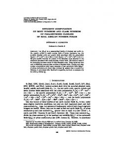
The computation of discrete approximations also provides an opportunity to detect patterns in the qualitative nature of the optimal solutions that can help in formulating educated guesses about the functional form of the optimal solutions to the infinite-dimensional problem (P∗ ) posed by the theory. In this section we focus on a simple example involving only two quality levels, where the buyers’ types are drawn from a uniform distribution. Formally, we have J = 2, F uniform on a rectangular support [v 1 , v 1 ] × [v 2 , v 2 ]. Figure 1 shows the graph of the buyer surplus U in (1), for a grid with T = 30. A reasonable visual “approximation” for the function U is the maximum of two onedimensional, strictly convex functions: one that depends only on v1 and the other that depends only on v2 . Moreover, these two functions meet along a linear path, on which U is non-differentiable. The solutions obtained by considering various values for the cost vector c, and various grid sizes, exhibited patterns that have prompted us to formulate the following simple mechanism as a candidate for a good approximation of the optimal solution in the infinite-dimensional 14

1 0.8

U

0.6 0.4 0.2 0 8 7.5

11 10.5

7

10

6.5

9.5

v1

6

9

v2

Figure 1: Buyer surplus function U for T = 30. problem (P∗ ). Consider the following class of mechanisms, parameterized by the “add-on price” p: Qp1 (v1 , v2 ) = F N −1 (v1 , v1 + p) 1 {v1 > v2 − p} Qp2 (v1 , v2 ) = F N −1 (v2 − p, v2 ) 1 {v1 < v2 − p} and

(Z p

U (v1 , v2 ; p) = max

v1

v1

Z Qp1 (t, v2 ) dt,

v2

v2

) Qp2 (v1 , t) dt

.

For any p, the mechanism (Qp , U p ) is feasible for the infinite-dimensional program (P∗ ), because it can be implemented by the following auction named “exclusive buyer mechanism”, for the case with two quality levels (see Brusco, Lopomo and Marx [4]). The buyers compete in a second-price or ascending-bid auction, possibly augmented with a reserve price r, for the right to be the only buyer who gets to choose between buying the object of lower quality (grade 1) at no additional cost, or the object of higher quality (grade 2) for an additional payment © ª of p.4 Since the value for buyer i ∈ N of winning the auction is β i ≡ max v1i , v2i − p , it is a dominant strategy for buyer i to bid β i at the auction. Thus, in equilibrium, buyer i wins © © ªª the auction only if β i ≥ max r, max β j ; j ∈ N \ {i} , is assigned the low-quality and high4

For the case with J > 2 quality levels, the winner of the auction selects a price-quality pair from a menu of up to J choices.

15

¢ ¡ ¢ ¡ quality object with probabilities Qp1 v1i , v2i and Qp2 v1i , v2i , respectively, and his expected utility is U p (v1 , v2 ; p). Let p∗ denote the value of p which maximizes the seller’s expected profit within the class of exclusive buyers mechanisms, i.e. across all values of p ∈ R. Table 3 shows how the value of the objective function in (P∗ ) evaluated at (Qp∗ , U p∗ ) (last row) compares with the values obtained by the objective function in (1) for various grid sizes, and F uniform on [v 1 , v 1 ] × [v 2 , v 2 ] = [6, 8] × [9, 11] , c1 = 0.9 and c2 = 5. J 2 2 2 2 2

N 2 2 2 2 2

T 5 10 20 30 1000∗

OPT VAL 6.051008 5.946440 5.896710 5.880743 5.838323

Table 3: Optimal values of (PT ) and the objective function value of the exclusive buyer mechanism (∗ obtained by numerical integration with T = 1000). As Table 3 shows, the exclusive buyer mechanism performs quite well relative to the numerical optimal solutions, at least for the case in which F is uniform. Moreover, as Figure 2 illustrates, the difference between the U function shown in Figure 1 and the buyer surplus function in the optimal exclusive buyer mechanism, for a grid of size T = 30, is relatively small. (The largest deviations occur near the “manifold” of non-differentiable points of U .) It is interesting to contrast the nature of the exclusive buyer mechanism with the qualitative features of the optimal mechanisms in the single buyer models, studied in Armstrong [1], Rochet and Chon´e [15], and Manelli and Vincent [8]. A main result in Armstrong [1] is that, in any optimal mechanism, it is optimal not to sell with positive probability. In contrast, in the optimal exclusive buyer mechanism with no reserve price, which performs quite well relative to the numerical optimal mechanisms in our numerical simulations, the object is always sold. Rochet and Chon´e [15] establish that “bunching is robust in these multidimensional screening problems, even with very regular distributions of types. This comes from a strong conflict between participation constraints and second order incentive compatibility conditions.” (Rochet and Chon´e [15]) Manelli and Vincent [8] reinforce the point that, in one buyer settings, optimal mechanisms are generically quite different in nature from the simple “take-it-or-leave-it” mechanisms, which are always optimal in the one-dimensional case: “We find that the set of extreme points contains, in addition to price-posting, many “novel” mechanisms. In particular, extreme points need not be simple functions 16

1

U T − U p∗

0.5

0

−0.5

−1 8

11 7.5

10.5 10

7

9.5

6.5

6

v1

9

v2

Figure 2: The difference between the buyer surplus function in (PT ), for T = 30, and the buyer surplus function in the optimal exclusive buyer mechanism. (Example 2), and even when they are, they may randomly assign objects to consumers (Examples 1 and 3). In contrast to the one-good case, the form of the optimal mechanism is determined by the prior distribution of buyer valuations.” (Manelli and Vincent [8]) In contrast, our analysis suggests that the exclusive buyer mechanism with an optimally chosen ‘add-on’ price can perform quite well, and shares many of its defining features with its one-dimensional counterparts, i.e. Myerson’s optimal auctions: there is no ‘bunching’, and is defined by simple rules that do not depend on the prior distribution of buyer valuations.

Appendix A.

Auxiliary Technical Results

Lemma 13 The inequalities in (C) are equivalent to the inequalities in (B). Proof. Using our notation, Proposition 3.1 in Border [3] states: Let X : V → [0, 1] be measurable. Then X is implementable by a symmetric auction if and only if for each measurable set A ⊂ T , the following inequality is satisfied: Z X (v) dF (v) ≤

1−

³R

V \A dF (v)

N

A

17

´N .

¡ ¢ By “X is implementable” Border means that there exists a symmetric function x = x1 , ..., xN : V N → [0, 1]N such that Z ³ ´ ¡ i¢ ¡ ¢ Y X v ≡ xi v i , v −i dF v k . V N −1

k∈N \{i}

The equivalence between (C) and (B) follows immediately from Border’s Proposition 3.1, by ¡ ¢ P ¡ ¢ P i letting xi (ω) = qj (ω) and X v i = Qj v i . j∈J

j∈J

Lemma 14 Let h be a Lipschitz function on V , with constant L, and let ˆ h(v) = {h(ˆ v ) : for some vˆ such that kv − vˆk ≤ ε} be a piecewise constant function. For any measurable function g : V → R we have that Z ¯ Z ¯ ¯ ¯ ˆ |g(v)|dv for any D ⊂ V. ¯h(v) − h(v)¯ g(v)dv ≤ Lε D

D

ˆ we have that |h(v) − h(v)| ˆ Proof. Since h is Lipschitz, by definition of h ≤ Lε. The result follows by integration. e T be defined Lemma 15 For some T > 0 consider the grid VT defined by ² = O(1/T ). Let U as in (1). For any v ∈ V we have that e T (v) − U e T (v 0 ) ≤ ², v 0 ∈ VT , v 0 ≤ v < v 0 + ²e. 0≤U e T is a convex function. By its definition, any subgradient of U e T belongs Proof. Note that U to the set conv{QT (v) : v ∈ VT }. It follows that any subgradient s ∈ conv{QT (v) : v ∈ VT } is such that s ≥ 0 and ° ° °X ° X ° ° T ° ° ≤ ksk1 ≤ max α Q (v) αv sup kQT (v)k1 ≤ 1. v P ° αv ≥0, v∈V αv =1 ° v∈VT °v∈VT ° T v∈VT 1

Thus, e T (v)−U e T (v 0 ) ≤ U

sup

­ ® | s, v − v 0 | ≤

e T (αv+(1−α)v 0 ) α∈[0,1],s∈∂ U

sup e T (αv+(1−α)v 0 ) α∈[0,1],s∈∂ U

Moreover, since s ≥ 0 and v − v 0 ≥ 0, we have e T (v) ≥ U e T (v 0 ) + hs, v − v 0 i ≥ U e T (v 0 ). U

18

ksk1 kv−v 0 k∞ ≤ ².

Lemma 16 Under Assumption 2 we have that ¯ ¯ Z X¯ √ ¯ 0 0 ¯fˆ(v) − f (v )dv ¯¯ ≤ 2² J sup k∇f (v)kvol(V ) ¯ 0 v∈V

v≤v ≤v+²e

v∈VT

Proof. For convenience let Cv = {v 0 ∈ V : v ≤ v 0 < v + ²e} where ² = O(1/T ). By the mean R value theorem, Cv f (v 0 )dv 0 = f (˜ v )²J where v˜ ∈ Cv . The triangular inequality yields ¯ Z X¯ ¯fˆ(v) − ¯ v∈VT

¯ ¯ ¯¶ Z Xµ ¯ ¯ J ¯ J 0 0¯ ˆ ¯ f (v )dv ¯ ≤ |f (v) − f (v)² | + ¯² f (v) − f (v )dv ¯ Cv Cv v∈VT ³ ´ X ≤ |fˆ(v) − f (v)²J | + ²J |f (v) − f (˜ v )| 0

0¯

v∈VT

Note that for the first term we have X v∈VT

¯ ¯ ¯ ¯ ¯ ¯ ¯ ¯ X X ¯ ¯ ¯ ¯ f (v) 0 J J J 0 ˆ ¯ ¯ ¯ P f (v )² ¯¯ 1−² f (v )¯ = ¯1 − |f (v) − f (v)² | = ¯ 0 ¯ ¯ ¯ v 0 ∈VT f (v ) ¯ v∈V v 0 ∈VT v 0 ∈V ¯T ¯ T ¯ ¯ X X ¯ ¯X f (v 0 )²J ¯¯ ≤ ²J |f (˜ v 0 ) − f (v 0 )| = ¯¯ f (˜ v 0 )²J − ¯ ¯v0 ∈VT v 0 ∈VT v 0 ∈VT X

Finally, we bound X

²J |f (v) − f (˜ v )| ≤

v∈VT

Appendix B.

X v∈VT

√ ­ ® ²J sup | ∇f (v 0 ), v − v˜ | ≤ ² J sup k∇f (v)kvol(V ). v 0 ∈Cv

v∈V

Proofs of Section 3

Proof of Theorem 4. Within this proof we omit the superscript T for notational convee is convex (since it is the maximum of affine functions) and nonnience. First note that U e (v) ≥ U (v) = 0. negative in V by construction since U To show (ii) consider any two points v, v 0 ∈ V and denote by vˆ, vˆ0 ∈ VT the points that vˆ ≤ v < ²e, and vˆ0 ≤ v 0 < vˆ0 + ²e. Next recall that all (IIC) are satisfied for all vˆ, vˆ0 ∈ VT . e e (ˆ e (ˆ Since Q(v) = Q(ˆ v ), U v ) = U (ˆ v ), U v 0 ) = U (ˆ v 0 ), we have D E e (v 0 ) − U e (v) − Q(v), e e (v 0 ) − U (ˆ e (v) + U (ˆ U v0 − v =U v 0 ) + U (ˆ v) − U v 0 ) − U (ˆ v ) − hQ(ˆ v ), v 0 − vi ≥ −² + hQ(ˆ v ), v 0 − vˆ0 + vˆ − vi + U (ˆ v 0 ) − U (ˆ v ) − hQ(ˆ v ), vˆ0 − vˆi ≥ −² − kQ(ˆ v )k1 kˆ v − vk∞ ≥ −2²,

19

e (v 0 ) ≥ U e (ˆ e e (v). by Lemma 15, U v 0 ), hQ(ˆ v ), v 0 − vˆ0 i ≥ 0, and kQ(ˆ v )k1 ≤ 1. Thus Q(v) ∈ ∂2² U Since violations to (IIC) are bounded by (ii), to show (iii) we need to control the violation among all Border constraints. By Lemma 9 it suffices to consider sets of the form Eα = {v ∈ P e j (v) ≥ α}. The definition of Q e implies that these sets are of the form unions of V : Jj=1 Q cubes of side ² (and therefore volume ²J ). Let A = ∪v∈AT ⊂VT {v 0 ∈ V : v ≤ v 0 < v + ²e}, then we have ¯ ¯ ¯Z X ¯ ¯Z ¯ X X X X ¯ ¯ ¯ ¯ 0 0 e ¯ Q(v)dF (v) − Q(v)fˆ(v)¯¯ ≤ Q(v) ¯¯ f (v )dv − fˆ(v)¯¯ ¯ v≤v 0 A dF (v). In turn this implies that   Hα =



v∈V :

X

  Qj (v) = α

j∈J



has positive measure with respect to F , that is Z Z Z dF (v) > dF (v) − dF (v) > 0. Hα

Eα

A

(Otherwise we would be able to choose a larger α.) Consider the violation of the Border constraint associated with A   µ ¶N Z X Z  δ A := Qj (v) dF (v) − 1 + 1 − dF (v) A

j∈J

Z δ(µ) := αµ + Eα \Hα

and

A

  Ã Z X  Qj (v) dF (v) − 1 + 1 −

!N dF (v) − µ

Eα \Hα

j∈J

R

where µ = H dF (v) with H ⊂ Hα . The latter is a convex function in the scalar µ ∈ R [0, Hα dF (v)] so it is maximized at one of the extremes (i.e., the extremes have a violation at least as big as δ A ). Note that there might be no set H associated with intermediate values R R of µ (say µ = A dF (v) − Eα \Hα dF (v)) but the maximum is achieved in the extreme. This allows us to obtain at least the same violation as δ A either with H = ∅ or H = Hα . These cases correspond to set of the form Eα . Proof of Lemma 10.

Regarding the separation oracle for (IIC) note that we can simply

23

enumerate them. Each of the O(T 2J ) constraint requires O(J) operations. Next we turn to Border constraints. Let (Q, U ) be the point to be considered by the oracle. First construct the O(T J )-dimensional vector Q defined as Q(v) =

X

Qj (v)

j∈J

which accounts for O(JT J ) operations. Then we sort the vector Q in descending order using b Next note that we can generate all the O(T J ) sets Eα O(T J ln(T J )) operations to create Q. associated with Q by considering the following sets of components {{1}, {1, 2}, {1, 2, 3}, . . . , {1, 2, . . . , O(T J )}} b Since this can be done incrementally, the computational cost to search over all these sets of Q. is O(T J ). Proof of Lemma 12. Let S k denotes the set of indices of included Border and IC constraints at the k-th iteration. Since there are a finite number of constraints, there is a finite number of possible sets S k each of which containing a finite number of extreme points or faces. Therefore there is only a finite number of different objective function values that can be achieved at any iteration. Since inequalities are discarded only if an improvement on the objective function is observed, either we keep accumulating inequalities or a improvement in the objective function is made.

References [1] Armstrong, M. (1996) “Multiproduct nonlinear pricing,” Econometrica 64-1: 51–75. [2] Besanko, D., S. Donnenfeld and L. White (1987), “Monopoly and Quality Distortion: Effects and Remedies,” Quarterly Journal of Economics, 102: 743-768 [3] Border K., (1991) “Implementation of reduced form auctions: a geometric approach,” Econometrica 59: 1175-1187. [4] Brusco, S. G. Lopomo and L. Marx (2008) “The Economics of Contingent Re-auctions” working paper, Duke University. [5] J.-B. Hiriart-Urruty and C. Lemar´echal. Convex Analysis and Minimization Algorithms. Number 305-306 in Grund. der math. Wiss. Springer-Verlag, 1993. (two volumes). [6] Gr¨otschel, M., L. Lov´asz, and A. Schrijver (1981). Geometric Algorithms and Combinatorial Optimization, Springer-Verlag, New York, NY. [7] Gr¨otschel, M., L. Lov´asz, and A. Schrijver (1988). The ellipsoid method and its consequences in combinatorial optimization, Combinatorica, 1, 169-197. 24

[8] Manelli A. and D. Vincent (2007) “Multidimensional Mechanism Design: Revenue Maximization and the Multiple-Good Monopoly,”, Journal of Economic Theory 137: 153-185. [9] Maskin, E. and J. Riley (1984) “Monopoly with Incomplete Information,” The Rand Journal of Economics 15-2: 171-196 [10] Maskin, E. and J. Riley (1986). “Optimal Auctions with Risk Averse Buyers”, Econometrica, Vol. 52, No. 6 (Nov., 1984), pp. 1473-1518. [11] Mussa M. and S. Rosen (1978) “Monopoly and Product Quality,” Journal of Economic Theory 18: 301-317. [12] Myerson, R. (1981) “Optimal Auction Design,” Mathematics of Operation Research 6: 58-73. [13] Myerson, R. (1979) “Incentive Compatibility and the Bargaining Problem,” Econometrica 47: 61-73. [14] Padberg, M. W., and M. R. Rao (1980). The Russian method and integer programming, working paper, New York University, New York, NY. [15] Rochet, J. and Chon´e, P. (1998) “Ironing, Sweeping, and Multidimensional Screening,” Econometrica, 66-4: 783-826. [16] Rockafellar, R. T., Convex Analysis, Princeton University Press, Princeton, NJ, 1970. [17] Wilson, R., Nonlinear Pricing, Oxford University Press, 1993.

25