finite element galerkin approach for a computational ...

Applied Mathematics and Mechanics ( English Edition , Vol 22 , No 9 , Sep 2001)

Published by Shanghai University , Shanghai , China

Article ID : 0253- 4827 ( 2001) 09- 1012- 07

FIN I TE EL EM EN T GAL ER KIN A P P ROA C H FO R A COM PU TA TIONAL S TU D Y O F A R TERIAL FLOW Ξ G. C. Sharma ( G. C. 夏玛) , 　Madhu J ain ( 马德胡・ 珍) , 　Anil Kumar ( 阿尼尔・ 克乌玛) ( School of Mathematical Sciences , Institute of Basic Science , Khandari , Agra-282002 , India) ( Communicated by CHIEN Wei- zang) A bst r act : A finite element solution for the Navier-Stokes equations for steady flow through a double branched two dimensional section of three dimensional model of canine aorta is obtained. The numerical technique involves transformation of the physical coordinates to a curvilinear boundary fitted coordinate system. The shear stress at the wall is calculated for Reynolds number of 1000 with branch to main aortic flow rate ratio as a parameter . The results are compared with earlier works involving experimental data and it is observed that the results are very close to their solutions . This work in fact is an improvement of the work of Sharma and Kapoor ( 1995) in the sense that computations scheme is economic and Reynolds number is large . Ke y wor ds : shear stress ; blood flow ; arterial flow ; Galerkin approach CL C n u m be rs : O242 . 21 ; O357 . 1 　　　Doc u me nt code : A

I nt rod ucti on The measurement of shear stress in arterial flow has been bestowed by nature because of the possible relation between the shear stress at the wall and existence of atherosclerosis . The flow phenomena in large and medium sized arteries influence the development of atherosclerosic damage. Atherosclerosis is degenerative disease caused by accumulation of lipids and other materials under the endothelial layers lining the arterial wall . These areas of collection are known as plaques . The greatest predilection for the disease is in proximity to bends , junctions and [1] branches of large arteries . Fry ( 1969) assumed that these plaques represent the tissue response [2] to an increased flux plasma substances across an endothelial surface . Thompson et al . ( 1974) considered a numerical technique for generating a natural coordinate system for an arbitrary [3] geometry. Gokhale et al . ( 1978 ) used the finite element method to solve the steady state [4] Navier- Stokes equations in a two dimensional section of geometry. Gresno et al . ( 1979 ) [5] solved the set of Navier- Stokes equations . Lutz et al . ( 1981) considered a simplifed model of a double branched network that shows the region from the thoracic aorta and includes the celaic [6] and mesntric branches . Mishra and Singh ( 1983 ) investigated the non- linear flow of blood [7] through arteries . Sharma and Kapoor ( 1995 ) studied mathematical analysis of blood flow

Ξ Recei ve d dat e : 2000- 03- 03 ; Re vis e d dat e : 2001- 07- 08 Fou n dati on it e m : CSIR , New Delhi ( 25/ 98/ 97- EMR- Ⅱ) 1012 © 1995-2004 Tsinghua Tongfang Optical Disc Co., Ltd. All rights reserved.

A Computational Study of Arterial Flow

1013

[8] through arteries . Dash et al . ( 1996) studied changed flow in a narrow artery and estimated the [9] increased friction in the artery due to catheterization. Ku ( 1997) did research in blood flow in [ 10 ] arteries Dash et al . ( 1999 ) made analysis of blood flow in catheterized curved artery with stenosis . The fluid is Newtonian and incompressible and the flow is assumed in the region of the arterial system. Here the numerical schemes involve first the transformation of coordinates and then resulting parameters are used in the Galerkin approach schemes . We used the Galerkin technique to compute the results and the shear stress at the wall is calculated for a Reynolds number of 1000 . It is found that the results are very close to the experimental results . The [7] numerical results are then compared with results of Sharma and Kapoor ( 1995) .

1 　Tra nsf or ma ti on of t he Coor di na t es The following elliptic equations are used to generate the boundary fitted coordinate system :

52ξ 52ξ 52η 52η + = 0. 2 + 2 = 0, 　 5x 5y 5 x2 5 y2

( 1 , 2)

These equations constitute a transformation from the physical plane to numerical plane . This transformation is governed by the elliptic equation , it is called elliptic grid generation [ Thompson ( 1974) ] [ 2 ] . Interchanging dependent and independent variables in Eqs . ( 1) and ( 2) we have 2 2 2 α 5 x2 - 2β 5 x + γ 5 x2 = 0 , ( 3)

5ξ

5ξ5η

5η

and 2 2 2 α 5 y2 - 2β 5 y + γ 5 y2 = 0 , 5ξ5η 5ξ 5η

( 4)

where α, β, γare coordinate transformation parameters and x , y being expressed as independent variables .

2 　Gove r ni ng Fi el d Eq ua ti ons In this investigation assumptions are that the fluid is incompressible , isothermal and Newtonian and the flow is steady and laminar. Even though the steady state is our aim , it is easier computationally to retain the unsteady state terms and we get the steady state solution asymptotically in time . The conservation of mass and time dependent Navier- Stokes equations in the primitive variables are replaced by the transport equations and the elliptic stream function which in Cartesian rectangular coordinates system are 2 2 5ω 5ω 5ω 1 5ω 5ω + u + v = 2 + 5t 5x 5y Re 5 x 5 y2

( 5)

ω = 5v + 5 u. 5x 5y

( 6)

and

The equation of continuity can be satisfied by the stream function Ψ by

ψ2 Ψ 52 Ψ ( 7) + = - ω. 5 x2 5 y2 The Eq. ( 5) can be transformed to the numerical plane (ξ,η) and on transformation we get ,

© 1995-2004 Tsinghua Tongfang Optical Disc Co., Ltd. All rights reserved.

G. C. Sharma , Madhu Jain and Anil Kumar

1014

5ω Yη( uω) ξ - Yξ( uω) η Xξ( vω) η - Xη( vω) ξ + + = 5t j j (α ωξ - 2βωξη + γωηξ + σ ωη + τ ωξ) ,

j2 Re

( 8)

and

αΨξξ - 2βΨξη + γΨηη + σΨη + τΨξ = - j2ω, 2 2 where Re is the Reynolds number , and σ = - j P ,τ = - j Q. 211 　I niti al con diti ons

( 9)

An initial vorticity distribution is necessary for the initial valued vorticity transport equation , since transient solutions are not interested in the time dependent solutions . A tentative initial stream function distribution is calculated by solving the potential flow equations . By applying no slip at the solid wall boundaries the initial vorticity distribution is defined. 212 　B ou n da r y con diti ons Since Ψ = constant i . e . no mass flux at solid boundaries , the boundary conditions at the wall can be derived from Eq. ( 9) as follows :

　　　　　　　　　　　Wwall = 　　　　　　　　　　　Wwall = -

γ j2

α j2

　　( along η = constant ) , 　　( along ξ = constant )

and

5Ψ = 0. 5η At the exist planes , a Neumann type condition is specified for the velocities and vorticity

5ω 52 Ψ = 0 , 　 2 = 0 　　( along η = constant ) , 5η 5η and

5ω 52 Ψ = 0 , 　 2 = 0 　　( along ξ = constant ) . 5ξ 5ξ s M e t hod ) 3 　N u me rical M e t hod ( Gal e r ki n ’ In Galerkin’ s method we have

∫EΦ dΩ = 0 , Ω

i

( 10)

where E is Residual functional Φi weighting function and Ψ ^ ( x , y ) approximate solution. Here n

Ψ ^ ( x , y) =

∑Φc . i i

i= l

Therefore from Eq. ( 7) , we have -

52 Ψ 52 Ψ ω = 0. 5 x2 5 y2

Now Residual function E =-

52 Ψ ^ 52 Ψ ^ - ω. 2 5x 5 y2

© 1995-2004 Tsinghua Tongfang Optical Disc Co., Ltd. All rights reserved.

( 11)

A Computational Study of Arterial Flow

1015

Then we put Galerkin’ s Integral in the form as given below , 52 Ψ ^ 52 Ψ ^ + + ω Φi d x d y = 0 . 2 Ω 5x 5 y2 Integrating by parts and using Green- Gauss theorem , we get ,

∫

5Ψ

5Ψ

5 Ψ 5Φi

5 Ψ 5Φi

∫ 5 x Φ d y + 5 y Φ d x +∫ 5 x 5 x + 5 y 5 y - ωΦ 5Ψ 5Ψ ∫5 xΦ cos ( n , x) d s + 5 yΦ cos ( n , y) d s + 5 Ψ 5Φ 5 Ψ 5Φ ∫ 5 x 5 x + 5 y 5 y - ωΦ d xd y = 0 , Ψ 5Φ 5 Ψ 5Φ 　　　　　　 5 ∫ 5 x 5 x + 5 y 5 y - ωΦ d xd y = 5Ψ 5Ψ ∫ 5 xΦ cos ( n , x) + 5 yΦ cos ( n , y) d s .

　　　　　　 -

i

Ω

i

Ω

i

Ω

i

d xd y =

i

i

i

i

Ω

i

i

i

Ω

i

Γ

i

( 12)

Replacing Ψ ^ in ( 12 ) by ( 11 ) results in linear simultaneous algebraic equations . To solve these equations the Succesive Over Relaxation method is used. From Eq. ( 5) , we have n

u =

∑uΦ ( x , y) , i

i

i =1 n

v =

∑vΦ ( x , y ) , i

i

i =1

Fig. 1

n

w =

∑

w iΦi ( x , y ) .

i =1

These equations would be used with the primitive variable Galerkin’ s method in the form

5ω 5ω 5ω Φ 1 + u + v d xd y = 5t 5x 5y i Re

∫ Ω

∫g ωΦ d xd y . 2

i

Ω

( 13)

Applying the Green- Causs theorem to right hand side of Eq. ( 13) and inserting the equations for u , v and w we find the finite element equation as Ai , j

5ωi + ( B i , j + Ci , j ) ωi = 5t

∫ΦΦ d s , Γ

j

x

( 14)

where

∫ΦΦ d x d y , 1 5Φ 5Φ 5Φ 5Φ = ∫Re 5 x 5 x + 5 y 5 y d x d y , 5Φ 5Φ = Φ u ∫ 5 x + v 5 y Φ d xd y ,

　　　　　　　　A i , j = 　　　　　　B i , j 　　　　　　Ci , j

Ω

i

j

i

j

i

j

Ω

i

i

5ω 　　　　　　Φx = =5t

j

j

i

cos ( n , x )

i

5ωi 5ωi . + cos ( n , y ) 5x 5y

These equations are the standard Galerkin finite element equations . Their solution can be obtained by the predictor- correcter method or by any other similar method.

© 1995-2004 Tsinghua Tongfang Optical Disc Co., Ltd. All rights reserved.

1016

G. C. Sharma , Madhu Jain and Anil Kumar

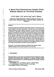
4 　Res ults a n d Disc ussi ons The numerical method was first tested by studying geometry considered by previous investigators . The natural coordinate lines generated by transforming the physical coordinates in Fig. 2 are shown Fig. 3 . The fluid mechanics problems are solved by Galerkin finite element scheme. Fig. 4 ( a ) and Fig. 4 ( b ) show comparison of the up stream and down stream wall vorticity distributions respectively.

　　　　　　　　　　　　　　　　　　　　　　　　Fig. 3 　Numerically generated curve 　　　　　　Fig. 2 　Single branch geometry linear coordinates lines

Fig. 4 ( a ) 　Wall vorticity distribution two dimensional artial flow

In the present work the flow parameter assumed is the branch to main flow rate ratio. The curves have the same profiles with shear rate values at the entering and exit for fully developed flow. But as shown the shear rate values reached a local maximum at one point and quickly dropped to zero or negative values before ascending at the exit point . The shear rate is maximum before bifurcation takes place , while at the bifurcation junction , since the stream is divided into two , the shear rate drops suddenly. The same thing happens when the next bifurcation takes place .

© 1995-2004 Tsinghua Tongfang Optical Disc Co., Ltd. All rights reserved.

A Computational Study of Arterial Flow

1017

Fig. 4 ( b) 　Wall vorticity distribution

Fig. 5 　Numerical steady flow velocity profiles

For the comparison numerical and experimental velocity vectors are shown in Fig. 5 and Fig. 6 respectively for a branch flow rate 20 %. In conclusion the numerical calculations of steady flow in the two dimensional model of the canine aorta are quite similar to the experimental results . Galerkin finite element scheme provided a good alternate to other methods for studying such

© 1995-2004 Tsinghua Tongfang Optical Disc Co., Ltd. All rights reserved.

1018

G. C. Sharma , Madhu Jain and Anil Kumar

Fig. 6 　Experimental steady flow velocity profiles

complex biological flow geometries . Other effects such as the pulsatile flow of elastic walls can be intimated into the basic approaches . In the final results , the numerical calculations of steady flow in the two dimensional model of the canine aorta are entirely similar to the experimental results . Ref e r e nces : [ 1 ] 　Fry D L . Certain histological and chemical responses of the vascular interface to acutely induced mechanical stress in the aorta of the dog [J ] . Circulation Res , 1969 , 93 - 108 . [ 2 ] 　Thompson J F , Thomes F C , Mastin C W. Automatic numerical generation of body-fitted curvilin2 ear coordinate system for field containing any of arbitrary two dimensional bodies [J ] . J Comput Phys , 1994 , 15 : 299 - 319 . [ 3 ] 　Gokhale V V , Tanner R I , Bischoff K B . Finite element solution of the Navier- Stokes equations for two dimensional steady flow through a section of a canine aorta model [J ] . J ournal of Biomechan2 ics , 1978 , 11 : 241 - 249 . [ 4 ] 　Gresho P M , Lee R L , Sani R L . Lawrence Livermore Laboratory Rept UCRL-83282 ,Sept , 1979 . [ 5 ] 　Lutz R J , Hsu L , Menawat A , et al . Fluid mechanics and boundary layer mass transport in an arte2 rial model during steady and unsteady flow [ A ] . In : 74 th Annual AICHE [ C ] . New Orleans , LA , 1981 . [ 6 ] 　Mishra J C , Singh S T. A large deformation analysis for aortic walls under a physiological loading [J ] . J Engg Sciences , , 1983 , 21 : 1193 - 1202 . [ 7 ] 　Sharma G C , Kapoor J . Finite element computation of two dimensional arterial flow in the presence of a transverse magnetic field [J ] . Internat J Numer Methods Fluids , 1995 , 20 : 1153 - 1161 . [ 8 ] 　Dash R K , Jayarman G , Mehta K M. Estimation of increased flow resistance in a narrow catheter2 ized arteries [J ] . J ournal of Biomechanics , 1996 , 29A :917 - 930 . [ 9 ] 　Ku N . Blood flow in arteries [J ] . Annual Review of Fluid Mechanics , 1997 , 29 : 399 - 434 . [ 10 ] 　Dash R K , Jayarman G , Mehta K M. Flow in cathertized curved artery with stenosis [J ] . J ournal of Biomechanics , 1999 , 32 : 46 - 61 .

© 1995-2004 Tsinghua Tongfang Optical Disc Co., Ltd. All rights reserved.