FINITE ELEMENT SUPG PARAMETERS COMPUTED FROM LOCAL

FINITE ELEMENT SUPG PARAMETERS COMPUTED FROM LOCAL DOF-MATRICES FOR COMPRESSIBLE FLOWS Lucia Catabriga Department of Computer Science, Federal University of Esp´ırito Santo (UFES) Av. Fernando Ferrari, s/n, Goiabeiras, 29060-900, Vit´oria, ES, Brazil [email protected] Alvaro L. G. A. Coutinho Department of Civil Engineering - COPPE, Federal University of Rio de Janeiro (UFRJ) Caixa Postal 68506, Rio de Janeiro, RJ, Brazil [email protected] Tayfun E. Tezduyar Team for Advanced Flow Simulation and Modeling (T*AFSM) Mechanical Engineering and Materials Science, Rice University MS 321 6100 Main Street, Houston TX 77005, USA [email protected] Abstract. For the SUPG formulation of inviscid compressible flows, we describe stabilization parameters defined based on the degree-of-freedom submatrices of the element-level matrices. In performance tests we compare these stabilization parameters with the ones defined based on the full element-level matrices. In both cases the formulation includes a shock-capturing parameter. We investigate the difference between updating the stabilization and shock-capturing parameters at the end of every time step and at the end of every nonlinear iteration within a time step. The formulation also involves activating an algorithmic feature that is based on freezing the shock-capturing parameter at its current value when a convergence stagnation is detected. Keywords: Euler equations, compressible flow, finite elements, element-by-element data structures, stabilization parameter

1.

INTRODUCTION

Stabilized formulations such as the streamline-upwind/Petrov-Galerkin (SUPG) (Hughes and Brooks 1979, Tezduyar and Hughes 1982, Tezduyar and Hughes 1983) and pressurestabilizing/Petrov-Galerkin (PSPG) (Tezduyar 1991) formulations are widely used in finite element flow computations. The SUPG and PSPG formulations prevent numerical oscillations and other instabilities in solving problems with high Reynolds and/or Mach numbers and shocks and strong boundary layers, as well as when using equal-order interpolation functions for velocity and pressure and other unknowns. It was pointed out in (Tezduyar et al. 1993) that these stabilized formulations also substantially improve the convergence rate in iterative solution of the large matrix systems that need to be solved at every Newton-Raphson step. The SUPG formulation for incompressible flows was first introduced in (Hughes and Brooks 1979). The SUPG formulation for compressible flows was first introduced, in the context of conservation variables, in (Tezduyar and Hughes 1982, Tezduyar and Hughes 1983). After that, several SUPG-like methods for compressible flows were developed. Taylor–Galerkin method (Donea 1984), for example, is very similar, and under certain conditions is identical, to one of the SUPG methods introduced in (Tezduyar and Hughes 1982, Tezduyar and Hughes 1983). Another example of the subsequent SUPG-like methods for compressible flows in conservation variables is the streamline-diffusion method described in (Johnson et al. 1984). Later, following (Tezduyar and Hughes 1982, Tezduyar and Hughes 1983), the SUPG formulation for compressible flows was recast in entropy variables and supplemented with a shockcapturing term (Hughes et al. 1987). It was shown in (Le Beau and Tezduyar 1991) that the SUPG formulation introduced in (Tezduyar and Hughes 1982, Tezduyar and Hughes 1983), when supplemented with a similar shock-capturing term, is very comparable in accuracy to the one that was recast in entropy variables. The PSPG formulation for the Navier–Stokes equations of incompressible flows, introduced in (Tezduyar 1991), assures numerical stability while allowing us to use equal-order interpolation functions for velocity and pressure. An earlier version of this stabilized formulation for Stokes flow was introduced in (Hughes et al. 1986). A stabilization parameter that is mostly known as “τ ” is embedded in the SUPG and PSPG formulations. This parameter involves a measure of the local length scale (also known as “element length”) and other parameters such as the local Reynolds and Courant numbers. Various element lengths and τ s were proposed starting with those in (Hughes and Brooks 1979) and (Tezduyar and Hughes 1982, Tezduyar and Hughes 1983), followed by the one introduced in (Tezduyar and Park 1986), and those proposed in the subsequently reported SUPG and PSPG methods. Here we will call the SUPG formulation introduced in (Tezduyar and Hughes 1982, Tezduyar and Hughes 1983) for compressible flows “(SU P G)82 ”, and the set of τ s introduced in conjunction with that formulation “τ82 ”. The stabilized formulation introduced in (Tezduyar and Park 1986) for advection–diffusion–reaction equations included a shock-capturing term and a τ definition that takes into account the interaction between the shock-capturing and SUPG terms. That τ definition precludes “compounding” (i.e. augmentation of the SUPG effect by the shock-capturing effect when the advection and shock directions coincide). The τ used in (Le Beau and Tezduyar 1991) with (SU P G)82 is a slightly modified version of τ82 . A shock-capturing parameter, which we will call here “δ91 ”, was embedded in the shock-capturing term used in (Le Beau and Tezduyar 1991). Subsequent minor modifications of τ82 took into account the interaction between the shock-capturing and the (SU P G)82 terms in a fashion similar to how it was done in (Tezduyar and Park 1986) for advection–diffusion– reaction equations. All these slightly modified versions of τ82 have always been used with the same δ91 , and we will categorize them here all under the label “τ82-MOD ”. Recently, new ways of computing the τ s based on the element-level matrices and vec-

tors were introduced in (Tezduyar and Osawa 2000) in the context of the advection–diffusion equation and the Navier–Stokes equations of incompressible flows. These new definitions are expressed in terms of the ratios of the norms of the relevant matrices or vectors. They automatically take into account the local length scales, advection field and the element-level Reynolds number. Based on these definitions, a τ can be calculated for each element, or even for each element node or degree of freedom or element equation. It was pointed out in (Tezduyar and Osawa 2000, Tezduyar 2001) that the τ s to be used in advancing the solution from time level n to n + 1 (including the τ embedded in the “LSIC stabilization” term, which resembles a discontinuity-capturing term) should be evaluated at time level n (i.e. based on the flow field already computed for time level n), so that we are spared from another level of nonlinearity. In (Catabriga et al. 2002), the τ definitions based on the element-level matrices were applied to the (SU P G)82 formulation for inviscid compressible flows supplemented with the shock-capturing term involving δ91 . In this paper, we apply to the same formulation the τ definitions based on the degree-of-freedom submatrices of the element-level matrices. We investigate the performance differences between these τ definitions, the τ definitions based on the full element-level matrices, and τ82-MOD . We also investigate the performance differences between updating the stabilization and shock-capturing parameters at the end of every time step and at the end of every nonlinear iteration within a time step. The formulation includes activating an algorithmic feature, which was introduced earlier and is based on freezing the shock-capturing parameter at its current value when a convergence stagnation is detected. 2.

EULER EQUATIONS

The system of conservation laws governing inviscid, compressible fluid flow are the Euler equations. These equations, restricted to two spatial dimensions, may be written in terms of conservation variables U = (ρ, ρu, ρv, ρe), as U,t + Fx,x + Fy,y = 0 on Ω × [0, T ]

(1)

where Fx and Fy are the Euler fluxes given elsewhere (Hirsh 1992), Ω is a domain in IR2 and T is a positive real number. We denote the spatial and temporal coordinates respectively by x = (x, y) ∈ Ω and t ∈ [0, T ], where the superimposed bar indicates set closure, and Γ is the boundary of domain Ω. Here ρ is the fluid density; u = (ux , uy )T is the velocity vector; e is the total energy per unit mass. We add to equation (1) the ideal gas assumption, relating pressure with the total energy per unit mass and kinetic energy. Alternatively, equation (1) may be written as, U,t + Ax U,x + Ay U,y = 0 on Ω × [0, T ] where Ai = 3.

∂Fi . ∂U

(2)

Associated to equation (2) we have proper boundary and initial conditions.

STABILIZED FORMULATION AND STABILAZATION PARAMETERS

Considering a standard discretization of Ω into finite elements, the (SU P G)82 formulation for the Euler equations in conservation variables introduced by (Tezduyar and Hughes 1982) and (Tezduyar and Hughes 1983) is written as, µ ¶ Z h ∂Uh h h ∂U W . + Ai dΩ + ∂t ∂xi Ω ¶ · ¸ µ nel Z nel Z h X X ∂Wh ∂Uh ∂Uh ∂Wh h ∂U h T δ91 . dΩ + + Ai . dΩ = 0(3) (Ak ) τ ∂xk ∂t ∂xi ∂xi ∂xi e e e=1 Ω e=1 Ω

where Wh and Uh , respectively the discrete weighting and test functions, are defined on standard finite element spaces. In (3) the first integral corresponds to the Galerkin formulation, the first series of element-level integrals are the SUPG stabilization terms, and the second series of element-level integrals are the shock-capturing terms added to the variational formulation to prevent spurious oscillations around shocks. The shock-capturing parameter, δ91 , is evaluated here using the approach proposed by (Le Beau and Tezduyar 1991). We define the following element-level matrices: Z ∂Uh Wh m: dΩ (4) ∂t Ωe ¶ Z µ ∂Wh h ∂Uh ∂Wh h ∂Uh dΩ (5) .Ax + .Ay ˜ c: ∂x ∂t ∂y ∂t Ωe ¶ Z µ h h h h ∂U h h ∂U W .Ax c: + W .Ay dΩ (6) ∂x ∂y Ωe ˜: k

∂Wh h h ∂Uh ∂Wh h h ∂Uh .Ax Ax + .Ax Ay + ∂x ∂x ∂x ∂y Ωe ¶ ∂Wh h h ∂Uh ∂Wh h h ∂Uh .Ay Ax + .Ay Ay dΩ ∂y ∂x ∂y ∂y

Z

µ

(7)

Considering the standard finite element approximation we have: Uh = Nv,

Wh = Nc,

Uh,t = Na

(8)

where v is the vector of nodal values of U (depending on time only), c is a vector of arbitrary constants, a is the time derivate of the v (a = dv ) and N is a matrix containing the space dt dependent shape functions. Restricting ourselves to linear triangles, the element shape functions may be represented in matrix form as, £ ¤ Ne = N 1 I N 2 I N 3 I (9) where N1 , N2 e N3 are the element shape functions and I is the identity matrix of order 4. It is useful to define the discrete local (element) gradient operator as, ¸ · · ¸ · ∂N ¸ 1 y I y I y I Bx 23 31 12 ∂x (10) B= = ∂N = By 2Ae x32 I x13 I x21 I ∂y

where Ae is the area of the element, xij = xi −xj , and yij = yi −yj for i, j = 1, 2, 3. Substituting the above relations into the weak formulation and proceeding in the standard manner we may arrive to the element matrices:   Z 2I I I e A  I 2I I  m = NT NdΩe = (11) 12 Ωe I I 2I ˜ c =

Z

 m1 m1 m1 1 (BTx Ahx N + BTy Ahy N)dΩe = m2 m2 m2  6 Ωe m3 m3 m3 

(12)

where m1 , m2 and m3 are given by, m1 = y23 Ax + x32 Ay m2 = y31 Ax + x13 Ay m3 = y12 Ax + x21 Ay

(13)

 c1 c2 c3 1 c= (NT Ax Bx + NT Ay By )dΩe = c1 c2 c3  6 1 2 3 Ωe c c c 

Z

(14)

and the submatrices c1 , c2 and c3 are, c1 = y23 Ax + x32 Ay c2 = y31 Ax + x13 Ay c3 = y12 Ax + x21 Ay

˜= k

Z

BT Ωe

·

Ax Ax Ax Ay Ay Ax Ay Ay

(15)

¸



 B11 B12 B13 1  B21 B22 B23  BdΩe = 4Ae B31 B32 B33

(16)

The submatrices in Eq.(16) are: B12 B13 B21 B23 B31 B32 B11 B22 B33

= y23 (y31 Axx + x13 Axy ) + x32 (y31 Ayx + x13 Ayy ) = y23 (y12 Axx + x21 Axy ) + x32 (y12 Ayx + x21 Ayy ) = y31 (y23 Axx + x32 Axy ) + x13 (y23 Ayx + x32 Ayy ) = y31 (y12 Axx + x21 Axy ) + x13 (y12 Ayx + x21 Ayy ) = y12 (y23 Axx + x32 Axy ) + x21 (y23 Ayx + x32 Ayy ) = y12 (y31 Axx + x13 Axy ) + x21 (y31 Ayx + x13 Ayy ) = −(B12 + B13 ) = −(B21 + B23 ) = −(B31 + B32 )

(17)

where Aij = Ai Aj for i, j = x, y. 3.1 Computing τ by element matrix norms We define the SUPG parameters from the element matrices as given in (Tezduyar and Osawa 2000), τS1 =

kck ˜ kkk

τS2 =

∆t kck 2 k˜ ck

(18)

where ∆t is the time step and kbk = max1≤j≤nee {|b1j | + |b2j | + . . . + |bnee ,j |}, nee is the number of element equations, that is, the number of element nodes times the number of degrees of freedom per node. We define the resulting SUPG parameter, as given in (Tezduyar and Osawa 2000), µ ¶−1/r 1 1 τSU P G = + r (19) r τS1 τS2 where r is an integer parameter.

3.2 Computing τ by dof element submatrix norms We can calculate a separate τ for each element matrix degree of freedom. The resulting stabilization tensor is,   τρ   τu  τ SU P G =  (20)   τv τe where the subindexes (ρ, u, v, e) are the primitive variables. Each τi can be calculated by τi =

µ

1 r τS1 i

+

1 r τS2 i

¶−1/r

τS1i =

kci k ˜i k kk

τS2i =

∆t kci k 2 k˜ ci k

(21)

˜i and ˜ where ∆t is the time step. ci , k ci are the submatrices of the element matrices for each degree of freedom i = ρ, u, v, e. Theses submatrices are defined by element matrix coefficients. Let a general degree of freedom be denoted by i. Then the corresponding element submatrix bi can be written as,   bp1 ,1 bp1 ,2 bp1 ,3 . . . bp1 ,10 bp1 ,11 bp1 ,12 (22) bi = bp2 ,1 bp2 ,2 bp1 ,3 . . . bp2 ,10 bp2 ,11 bp2 ,12  bp3 ,1 bp3 ,2 bp3 ,3 . . . bp3 ,10 bp3 ,11 bp3 ,12 where if if if if

i=ρ i=u i=v i=e

then then then then

(p1 , p2 , p3 ) ≡ (1, 5, 9) (p1 , p2 , p3 ) ≡ (2, 6, 10) (p1 , p2 , p3 ) ≡ (3, 7, 11) (p1 , p2 , p3 ) ≡ (4, 8, 12)

(23)

The norms of these submatrices, used in (21) are computed by kbi k = max1≤j≤nee {|bp1 ,j | + |bp2 ,j | + |bp3 ,j |}. 4.

NUMERICAL RESULTS

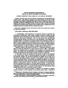
In this section we report numerical test results obtained with various stabilization parameters. The symbol τg represents τ calculated based on the element-level matrices, and the symbol τdof represents τ calculated based on the degree-of-freedom submatrices of the element-level matrices. We also test different update strategies for τ s and δ91 . In all test computations the number of multicorrections is 3. For the GMRES iterations, the dimension of the Krylov subspace is 5 and the tolerance is 0.1. All solutions are initialized with the free-stream values. 4.1 Oblique Shock The first problem consists of a two-dimensional steady problem of a inviscid, Mach 2, uniform flow, over a wedge at an angle of −10◦ with respect to a horizontal wall, resulting in the occurrence of an oblique shock with an angle of 29.3◦ emanating from the leading edge of the wedge, as shown in Fig. 1. The computational domain is the square 0 ≤ x ≤ 1 and 0 ≤ y ≤ 1. Prescribing the following flow data at the inflow, i.e., on the left and top sides of the shock, results in the exact

y x = 0.9

M = 2.0

M = 1.64052 29.3 ο

x

Figure 1: Oblique shock – problem description.

solution with the flow data past the shock:   M = 2.0      = 1.0 ρ Inflow Outflow u1 = cos100   0  u2 = −sin10    p = 0.17857

  M      ρ u1    u2    p

= = = = =

1.64052 1.45843 0.88731 0.0 0.30475

(24)

where M is the Mach number, ρ is the flow density, u1 and u2 are the horizontal and vertical velocities respectively, and p is the pressure. Four Dirichlet boundary conditions are imposed on the left and top boundaries; the slip condition u2 = 0 is set at the bottom boundary; and no boundary conditions are imposed on the outflow (right) boundary. A 20 × 20 mesh with 800 linear triangles and 441 nodes is employed. Figure 2(a) and 2(c) show, respectively, density along line x = 0.9 and the evolution of density residual for 300 steps, computed with τ82-MOD , τg and τdof , with r = 2. Here we update τg , τdof and δ91 at every nonlinear iteration of a time level (i.e. iteration update). We also tested what happens if we update τdof , τg and δ91 only at every time step at the beginning of a time step (i.e. time-step update), the results are in Fig. 2(b) and 2(d). The evolution of density residual for time-step update is faster than iteration update. Figure 3 shows the action of a procedure (Catabriga and Coutinho 2002) detecting convergence stagnation and freezing the shock-capturing parameter, with the two update strategies for τ82-MOD , τg and τdof stabilization parameters and δ91 shock-capturing parameter. Table 1 shows the number of GMRES iterations (NGM RES ) and number of steps (Nsteps ) for both update schemes. The results with τdof need less steps than the other alternatives, but more GMRES iterations. Note too that τ82-MOD needs more steps than all others. Results with time-step update are similar, but less steps are required. 4.2 Reflected Shock This two-dimensional steady problem consists of three regions (R1, R2 and R3) separated by an oblique shock and its reflection from a wall, as shown in Fig. 4. Prescribing the following Mach 2.9 flow data at the inflow, i.e., the first region on the left (R1), and requiring that the

1.6

1.6

τ82-MOD τg τdof

1.5

τ82-MOD τg τdof

1.5

exact

1.4

1.4

1.3

1.3

1.2

1.2

1.1

1.1

1

1

0.9

0.9

0.8

exact

0.8 0

0.2

0.4

0.6

0.8

1

0

(a) Density profile at x = 0.9 – iteration update 0.1

0.2

0.4

0.6

0.01

0.01

0.001

0.001

0.0001

0.0001

1e-05

1

(b) Density profile at x = 0.9 – time-step update 0.1

τ82-MOD τg τdof

0.8

τ82-MOD τg τdof

1e-05 0

50

100

150

200

250

300

350

0

50

100

150

200

250

300

350

(c) Evolution of density residual – iteration update (d) Evolution of density residual – time-step update

Figure 2: Oblique shock – solutions and residuals with iteration update and time-step update – using τ82-MOD , τg and τdof .

Table 1: Oblique shock – computational costs (in number of GMRES iterations and time steps) with iteration update and time-step update (both with freezing shock-capturing parameter) – using τ82-MOD , τg and τdof .

Update Iteration Time-step

τ82-MOD NGM RES Nsteps 5,226 869 5,289 861

τg NGM RES Nsteps 4,287 846 4,246 838

τdof NGM RES Nsteps 4,902 833 4,857 819

1.6

1.6

τ82-MOD τg τdof

1.5

τ82-MOD τg τdof

1.5

exact

1.4

1.4

1.3

1.3

1.2

1.2

1.1

1.1

1

1

0.9

0.9

0.8

exact

0.8 0

0.2

0.4

0.6

0.8

1

(a) Density profile at x = 0.9 – iteration update 0.1

τ82-MOD τg τdof

0.01

0

0.4

0.6

0.8

1

(b) Density profile at x = 0.9 – time-step update 0.1

τ82-MOD τg τdof

0.01

0.001

0.001

0.0001

0.0001

1e-05

1e-05

1e-06

1e-06

1e-07

1e-07

1e-08

1e-08

1e-09

1e-09

1e-10

1e-10

1e-11

0.2

1e-11 0

100 200 300 400 500 600 700 800 900

0

100 200 300 400 500 600 700 800 900

(c) Evolution of density residual – iteration update (d) Evolution of density residual – time-step update

Figure 3: Oblique shock – solutions and residuals with iteration update and time-step update (both with freezing shock-capturing parameter) – using τ82-MOD , τg and τdof .

incident shock to be at an angle of 29◦ , leads to the exact solution (R2 and R3):    M = 1.94235 M = 2.3781 M = 2.9              ρ = 2.68728  ρ = 1.7  ρ = 1.0 R3 u1 = 2.40140 R2 u1 = 2.61934 R1 u1 = 2.9       u = 0.0 u2 = −0.50632 u2 = 0.0        2   p = 2.93407 p = 1.52819 p = 0.714286

(25)

y M=2.3781 29 ο

M=1.94235

M=2.9 2 y=0.25

1

3 ο 23.28

x

Figure 4: Reflected shock – problem description.

We prescribe density, velocities and pressure on the left and top boundaries; the slip condition is imposed on the wall (bottom boundary); and no boundary conditions are set on the outflow (right) boundary. We consider a structured mesh with 60 × 20 cells, where each cell was divided into two triangles (1281 nodes and 2400 elements) and an unstructured mesh with 1,837 nodes and 3,429 elements covering the domain 0 ≤ x ≤ 4.1 and 0 ≤ y ≤ 1. Figure 5(a) and 5(b) show the density along line y = 0.25 for the structured mesh, computed by a τ82-MOD parameter, τg parameter and τdof , respectively, for iteration update and timestep update, both with r = 2. The density profile with τdof and time-step update shows some discrete oscillations. The evolution of density residual for 300 steps can be observed in Fig. 5(c) and 5(d). We observe that the density residual computed updating τg , τdof and δ91 with time-step update is smaller than the one computed by iteration update. Figure 6 shows the action of the convergence stagnation detection procedure, with the two updating strategies for τg , τdof and δ91 . In Fig. 6(a) and 6(b) we can observe the density profiles computed with the convergence stagnation procedure switched on are very similar to the previous cases. However, here τ82-MOD lead to a better evolution of the density residual (6(c) and 6(d)). We may see in Table 2 that here τ82-MOD solution required less steps for both update schemes. It is also interesting to note that τg and τdof solutions were more sensitive to the particular update scheme, with better results for time-step update. Table 2: Reflected shock (with structured mesh) – computational costs (in number of GMRES iterations and time steps) with iteration update and time-step update (both with freezing shock-capturing parameter) – using τ82-MOD , τg and τdof .

Update Iteration Time-step

τ82-MOD NGM RES Nsteps 3,226 531 3,180 512

τg NGM RES Nsteps 3,368 582 3,073 518

τdof NGM RES Nsteps 3,743 625 3,382 570

Figures 7 and 8 show the results for the unstructured mesh, computed by using the same τ s and update strategies of the previous case. The action of the convergence stagnation detection

τ82-MOD τg τdof

3

τ82-MOD τg τdof

3

exact

2.5

2.5

2

2

1.5

1.5

1

1

0.5

exact

0.5 0

0.5

1

1.5

2

2.5

3

3.5

4

(a) Density profile at y = 0.25 – iteration update. 0.1

0

0.5

1

1.5

2

2.5

0.01

0.01

0.001

0.001

0.0001

0.0001

1e-05

3.5

4

(b) Density profile at y = 0.25 – time-step update. 0.1

τ82-MOD τg τdof

3

τ82-MOD τg τdof

1e-05 0

50

100

150

200

250

300

350

0

50

100

150

200

250

300

350

(c) Evolution of density residual – iteration update. (d) Evolution of density residual – time-step update.

Figure 5: Reflected shock (with structured mesh) – solutions and residuals with iteration update and time-step update – using τ82-MOD , τg and τdof .

τ82-MOD τg τdof

3

τ82-MOD τg τdof

3

exact

2.5

2.5

2

2

1.5

1.5

1

1

0.5

exact

0.5 0

0.5

1

1.5

2

2.5

3

3.5

4

(a) Density profile at y = 0.25 – iteration update 0.1

0.5

1

1.5

2

2.5

3.5

4

τ82-MOD τg τdof

0.01

0.001

0.001

0.0001

0.0001

1e-05

1e-05

1e-06

1e-06

1e-07

1e-07

1e-08

1e-08

1e-09

1e-09

1e-10

1e-10

1e-11

3

(b) Density profile at y = 0.25 – time-step update 0.1

τ82-MOD τg τdof

0.01

0

1e-11 0

100

200

300

400

500

600

700

0

100

200

300

400

500

600

(c) Evolution of density residual – iteration update (d) Evolution of density residual – time-step update

Figure 6: Reflected shock (with structured mesh) – solutions and residuals with iteration update and time-step update (both with freezing shock-capturing parameter) – using τ82-MOD , τg and τdof .

procedure can be observed. We see that the steady-state density distributions are in good agreement. We may see im Table 3 that for the unstructured mesh results with τdof are slightly better than all others for both update schemes.

(a) Iteration update – using τ82-MOD

(b) Time-step update – using τ82-MOD

(c) Iteration update – using τg

(d) Time-step update – using τg

(e) Iteration update – using τdof

(f) Time-step update – using τdof

Figure 7: Reflected shock – density computed with iteration update and time-step update (both with freezing shock-capturing parameter) – using τ82-MOD , τg and τdof . 0.1

τ82-MOD τg τdof

0.01

0.1 0.01

0.001

0.001

0.0001

0.0001

1e-05

1e-05

1e-06

1e-06

1e-07

1e-07

1e-08

1e-08

1e-09

1e-09

1e-10

1e-10

1e-11

τ82-MOD τg τdof

1e-11 0

100 200 300 400 500 600 700 800 900

0

100 200 300 400 500 600 700 800 900

(a) Evolution of density residual – iteration update. (b) Evolution of density residual – time-step update.

Figure 8: Reflected shock (with unstructured mesh) – residuals with iteration update and time-step update (both with freezing shock-capturing parameter) – using τ82-MOD , τg and τdof .

5.

CONCLUDING REMARKS

We described, for the SUPG formulation of inviscid compressible flows, stabilization parameters defined based on the degree-of-freedom submatrices of the element-level matrices. These definitions are expressed in terms of the ratios of the norms of the relevant matrices, and take automatically into account the flow field, the local length scales, and the time step size. By inspecting the solution quality and convergence history, we compared these stabilization

Table 3: Reflected shock (with unstructured mesh) – computational costs (in number of GMRES iterations and time steps) with iteration update and time-step update (both with freezing shock-capturing parameter) – using τ82-MOD , τg and τdof .

Update Iteration Time-step

τ82-MOD

τg

τdof

NGM RES Nsteps 9,573 836 9,977 857

NGM RES Nsteps 9,127 844 9,913 893

NGM RES Nsteps 9,138 845 9,278 817

parameters with the ones defined based on the full element-level matrices. In both cases the formulation includes a shock-capturing parameter. Also by inspecting the solution quality and convergence history, we investigated the performance difference between updating the stabilization and shock-capturing parameters at the end of every time step and at the end of every nonlinear iteration within a time step. The formulation also involves activating an algorithmic feature that is based on freezing the shock-capturing parameter at its current value when a convergence stagnation is detected. We observe that in all cases the solution qualities are very comparable. In terms of computational efficiency, τ definitions based on the degree-of-freedom submatrices and full element-level matrices show comparable performances. 6.

ACKNOWLEDGMENTS

This work is partly supported by grant CNPq/MCT 522692/95-8. The third author was supported by the US Army Natick Soldier Center and NASA. REFERENCES Catabriga, L., A. L. G. A. Coutinho and T.E. Tezduyar (2002). Finite element supg parameters computed from local matrices for compressible flows. In: 9th Brazilian Congress of Thermal Engineering and Sciences CD-ROM. Caxambu, Minas Gerais, Brazil. pp. 1–11. Catabriga, L. and A. L. G. A. Coutinho (2002). Improving convergence to steady-state of implicit SUPG solution of Euler equations. Communications in Numerical Methods in Engineering 18, 345–353. Donea, J. (1984). A Taylor-Galerkin method for convective transport problems. International Journal for Numerical Methods in Engineering 20, 101–120. Hirsh, C. (1992). Numerical Computation of Internal and External Flows - Computational Methods for Inviscid and Viscous Flows, Vol. 2. John Wiley and Sons Ltd. Chichester. Hughes, T. J. R. and A. N. Brooks (1979). A multi-dimensional upwind scheme with no crosswind diffusion. In: Finite Element Methods for Convection Dominated Flows (T.J.R. Hughes, Ed.). Vol. 34. ASME. New York. pp. 19–35. Hughes, T. J. R., L. P. Franca and M. Balestra (1986). A new finite element formulation for computational fluid dynamics: V. Circumventing the Babuˇska–Brezzi condition: A stable Petrov–Galerkin formulation of the Stokes problem accommodating equal-order interpolations. Computer Methods in Applied Mechanics and Engineering 59, 85–99. Hughes, T. J. R., L. P. Franca and M. Mallet (1987). A new finite element formulation for computational fluid dynamics: VI. Convergence analysis of the generalized SUPG formu-

lation for linear time-dependent multi-dimensional advective-diffusive systems. Computer Methods in Applied Mechanics and Engineering 63, 97–112. Johnson, C., U. Navert and J. Pitkaranta (1984). Finite element methods for linear hyperbolic problems. Computer Methods in Applied Mechanics and Engineering 45, 285–312. Le Beau, G. J. and T. E. Tezduyar (1991). Finite element computation of compressible flows with the SUPG formulation. In: Advances in Finite Element Analysis in Fluid Dynamics (M.N. Dhaubhadel, M.S. Engelman and J.N. Reddy, Eds.). Vol. 123. ASME. New York. pp. 21–27. Tezduyar, T. E. (1991). Stabilized finite element formulations for incompressible flow computations. Advances in Applied Mechanics 28, 1–44. Tezduyar, T. E. (2001). Adaptive determination of the finite element stabilization parameters. In: European Congress on Computational Methods in Applied Sciences and EngineeringECCOMAS Computational Fluid Dynamics Conference CD-ROM. Swansea, Wales, UK. pp. 1–13. Tezduyar, T. E. and T. J. R. Hughes (1982). Development of time-accurate finite element techniques for first-order hyperbloic systems with particular emphasis on the compressible Euler equations. NASA Technical Report NASA-CR-204772. NASA. Tezduyar, T. E. and T. J. R. Hughes (1983). Finite element formulations for convection dominated flows with particular emphasis on the compressible Euler equations. In: 21st Aerospace Sciences Meeting. Vol. 83-0125. AIAA. Reno, Nevada. Tezduyar, T. E. and Y. Osawa (2000). Finite element stabilization parameters computed from element matrices and vectors. Computer Methods in Applied Mechanics and Engineering 190, 411–430. Tezduyar, T. E., S. Aliabadi, M. Behr, A. Johnson and S. Mittal (1993). Parallel finite-element computation of 3D flows. IEEE Computer 26, 27–36. Tezduyar, T.E. and Y.J. Park (1986). Discontinuity capturing finite element formulations for nonlinear convection-diffusion-reaction problems. Computer Methods in Applied Mechanics and Engineering 59, 307–325.