Finite Index Subgroups of R. Thompson's Group F

arXiv:0711.1014v1 [math.GR] 7 Nov 2007

Finite Index Subgroups of R. Thompson’s Group F Collin Bleak and Bronlyn Wassink

ABSTACT: The authors classify the finite index subgroups of R. Thompson’s group F . All such groups that are not isomorphic to F are non-split extensions of finite cyclic groups by F . The classification describes precisely which finite index subgroups of F are isomorphic to F , and also separates the isomorphism classes of the finite index subgroups of F which are not isomorphic to F from each other; characterizing the structure of the extensions using the structure of the finite index subgroups of Z × Z.

1

Introduction

In this paper, we classify the finite index subgroups of R. Thompson’s group F . By this classification, we are able to answer Victor Guba’s Question 4.5 in the problems report [7]. The group F was introduced by R. Thompson in the late 1960’s as part of a family of groups F ≤ T ≤ V . It has been the object of much study, and it’s theory has impacted various fields of mathematics, including not only the theory of infinite groups, but also low-dimensional topology, simple homotopy theory, measure theory, and even category theory. An introductory reference to the theory of F , T , and V is the survey paper [6]. The main characterization of F that we will use is that it is the group of all piecewise-linear, orientation-preserving homeomorphisms of the unit interval which admit finitely many breaks in slope, where these breaks are restricted to occur over the diadic rationals Z[1/2], and where all slopes of affine segments of the graphs of these elements are integral powers of two. We will also use some of the standard presentations for F in our analysis, which presentations will be given in the next section. We will use the notation F IF to represent the set of all finite index subgroups of F . In order to state our results in full, we will need to build a specific homomorphism. Given f ∈ F , we will denote the derivative of f at x by f ′ (x), if it exists. We will also define f ′ (0) to be the derivative from the right at 0, and f ′ (1) 1

to be the derivative from the left at 1. Note that these last two derivatives always exist as elements of F are affine near 0 and 1 in (0, 1). We now define a well known homomorphism φ : F → Z 2 by the rule φ(f ) = (log2 (f ′ (0)), log 2 (f ′ (1))) for all f ∈ F . By a standard fact in the literature of F (Theorem 4.1 from [6]), the group commutator subgroup F ′ of F consists of precisely the elements in F with leading and trailing slopes one, that is, F ′ is the kernel of the map φ. ˜ (a,b) = h(a, 0), (0, b)i ≤ Given two positive integers a and b, we define K 2 Z . We now define ˜ (a,b) ). K(a,b) = φ−1 (K In particular, K(a,b) can be thought of as the group of all elements in F with graphs having slopes near zero as integral powers of 2a while at the same time having slopes near one as integral powers of 2b . We will call any such K(a,b) ≤ F a rectangular subgroup of F , or simply a rectangular group. We ˜ (a,b) ≤ Z 2 as rectangular groups, where the will also refer to the groups K context will make clear which sort of rectangular groups we are refering to. We are now ready to give an explicit list of our results. Our first theorem is a corollary of our last theorem, but as we will prove it earlier in the paper in a direct fashion, we will list it here as a stand-alone result. Theorem 1.1 Let H ∈ F IF . H is isomorphic to F if and only if H = K(a,b) for some positive integers a and b. Given positive integers a and b, it is immediate that F/K(a,b) ∼ = Za × Zb , in particular we have the following theorem. Theorem 1.2 Given any positive integers a and b, F can be regarded as a non-split extension of Za × Zb by F . In particular, there are maps ι and τ so that the following sequence is exact. 1

/F

ι

/F

τ

/ Za × Zb

/ 1.

We will prove two further theorems. Before stating them, we mention some key lemmas, and build some language that will help with the statements of the theorems. Lemma 1.3 If H ∈ F IF then F ′ ≤ H. 2

Once the previous lemma is established, it is not hard to come to the following lemma. Lemma 1.4 If H ∈ F IF then H P F . Now, the above lemmas assure us that we can analyze all of the finite index subgroups of F by considering the finite index subgroups of Z 2 . We have one further lemma, which will assist us in our statements below. Lemma 1.5 Suppose H ∈ F IF . There exist rectangular groups Inner(H) and Outer(H) so that Inner(H) is a unique maximal rectangular subgroup in H and Outer(H) a unique minimal rectangular group containing H. In particular, if H ∈ F IF , then we have the following list of containments (where the first two are equalities in the case that H is a rectangular group). Inner(H) P H P Outer(H) P F We are now in a position to state our next theorem. Theorem 1.6 1. The map φ induces a one-one correspondence between the finite index subgroups of F and the finite index subgroups of Z 2 . ˜ = φ(H) ≤ Z 2 , 2. Suppose H is a finite index subgroup of F , with image H and that a and b are positive integers so that Inner H = K(a,b) ≤ H. If ˜ K ˜ (a,b) , then Q is finite cyclic, and there are maps ι, ρ, ˜ι and Q = H/ ρ˜ so that the diagram below commutes with the two rows being exact: F ∼ =

1

 / K(a,b)

ι

φ|K(a,b)

/K ˜

ρ

/Q

/1

/Q

/ 1.

φ|H



1

/H

˜ ι

(a,b)

 / ˜ H

ρ˜

The essence of the above theorem is that in Z 2 , each finite index sub˜ is a finite cyclic extension (by Q above) of the maximal rectangular group H ˜ The extension pulls back, so that the finite index subgroup subgroup of H. H of F can be seen as a finite cyclic extension of the maximal rectangular group K(a,b) in H by the same group Q . Whenever Q is non-trivial, the 3

resulting extension is non-split and results in a group that is not isomorphic with F . We will give several examples at the end of the paper where Q above is non-trivial, that is, examples of finite index subgroups of F which are not isomorphic to F . We define Res: F IF → N , where we use the rule H 7→ n, where n is the cardinality of H/ Inner(H). We will call the value n in the last sentence the residue of H. It turns out the relationship between a finite index subgroup of F and its maximal rectangular subgroup is very special. We show the following lemma. Lemma 1.7 Suppose H, H ′ ∈ F IF , K = Inner(H), K ′ = Inner(H ′ ), and ξ : H → H ′ is an isomorphism. Then 1. ξ(K) = K ′ 2. K is characteristic in H and K ′ is characteristic in H ′ , and 3. Res(H) = Res(H ′ ). Note that in the above, the second two points follow easily from the first. For convenience, given a, b positive integers, let us fix a particular isomorphism τ(a,b) : K(a,b) → F , so that if f ∈ K(a,b) with φ(f ) = (as, bt) then φ(τ(a,b) (f )) = (s, t). (We note that these are the precise sorts of isomorphisms which we build in the proof of Theorem 1.1.) We also need to name the isomorphism Rev: F → F which is obtained if we conjugate the elements of F by the orientation-reversing map rev: [0, 1] → [0, 1] defined by the equation rev(x) = 1 − x. We are now ready to state our final theorem. Theorem 1.8 Suppose H, H ′ are finite index subgroups of F . Let a, b, c, d be positive integers so that K(a,b) = Outer(H), K(c,d) = Outer(H ′ ). H is isomorphic with H ′ if and only if τ(a,b) (H) = τ(c,d) (H ′ ) or τ(a,b) (H) = Rev(τ(c,d) (H ′ )). These investigations were started when Jim Belk asked the first author if he knew whether or not [the group we call K(2,2) ] is isomorphic to F . The approach taken in this paper was motivated by the proof of Brin’s ubiquity result (see [2]), where Brin shows that a subgroup of the full group of piecewise-linear, orientation-preserving homeomorphisms of [0, 1] contains a copy of R. Thompson’s group F if certain weak geometric conditions are satisfied. 4

We are unaware of any published results relating to our own work here. However, Burillo, Cleary and R¨ over, in the course of their investigations into the abstract commensurator of F , and using techniques different from our own, have also understood the one-one correspondence between the finite index subgroups of Z 2 and the finite index subgroups of F . Also, they have the result that the rectangular subgroups of F are isomorphic to F . See [5]. The authors would like to thank Matt Brin for interesting discussions of these results, and also for some observations and questions which helped us to refine the results. Also, the first author would like to thank Jim Belk for asking the initial question that lead to this work, and to thank Mark Brittenham, Ken Brown, Ross Geoghegan, Susan Hermiller, and John Meakin for interesting conversations about these results.

2

Definitions and Notation

Richard Thompson’s Group F can also described by the following presentations. F ∼ = hx0 , x1 , x2 , ... | xxj i = xj+1 for i < ji 2

x0 −1 x0 F ∼ = hx0 , x1 | [x0 x−1 1 , x1 ] = [x0 x1 , x1 ] = 1i

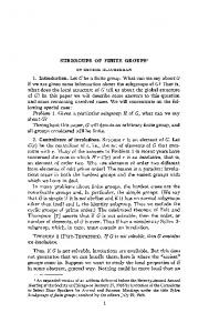
where ab = b−1 ab and [a, b] = aba−1 b−1 . In these presentations, the generators x0 and x1 can be realized as piecewise-linear homeomorphisms of the unit interval with breaks in slope occurring over the diadic rationals, and with all slopes being integral powers of two (that is, as elements of F using the definition of F as a group of homeomorphisms of the unit interval). We establish the mechanism of specifying any such function by listing the points in its graph where slope changes. We will call such points breaks, so that we will specify an element of F by listing its set of breaks. Let f0 be the element with breaks {(1/4, 1/2), (1/2, 3/4)} and let f1 be the element with breaks {(1/2, 1/2), (5/8, 3/4), (3/4, 7/8)}. The functions f0 and f1 play the roles of x0 and x1 in the presentations above. Here are the graphs of these functions.

5

f0

f1

Note that in the above, composition and evaluation of functions in F will be written in word order. In other words, if f, g ∈ F and t ∈ [0, 1] , then, tf = f (t), f g = g ◦ f , and f g = g−1 f g = g ◦ f ◦ g−1 . One can check, using the convention above, that f0 ∼ x0 and f1 ∼ x1 satisfy the relevant relations from the second presentation. It is well known that the second presentation is derived from the first (see [6] Theorem 3.4). The fact that f0 and f1 generate all of the claimed functions in F (as a group of homeomorphisms) is Corollary 2.6 in [6]. (Note that our functions f0 and f1 are the inverses of the homeomorphisms they use.) Given a homeomorphism f : [0, 1] → [0, 1], we will denote by Supp(f ) the support of f , wehre we take this set to be the set of all points in [0, 1] which are moved by the action of f . That is Supp(f ) = {x ∈ [0, 1]|xf 6= f } . (Note that this is different from the definition used in analysis, where a closure is taken.) The fact that elements of F have piecewise-linear graphs that admit only finitely many breaks in slope immediately implies that if f ∈ F , then Supp(f ) is a finite union of disjoint open intervals. We will call each of these disjoint open intervals an orbital of f .

3

Previous Results

Here we mention several lemmas necessary for our proof whose statements and proofs are spread throughout the literature. (If we do not give an indication of where a lemma may be found in the literature, then the lemma is standard and simple, and its proof may be taken as an exercise for the reader.)

6

Lemma 3.1 If f and g are set functions where the support of f is disjoint from the support of g, then f and g commute. Lemma 3.2 Let g, f ∈ F . Let H be the subgroup of F that is generated by f and g and define Supp(H) = {x ∈ [0, 1]|xh 6= x for some h ∈ H} . Then, Supp(H) = Supp(g) ∪ Supp(f ). The first point in the following lemma is essentially standard from the theory of permutation groups. It is stated (basic fact (1.1.a)) in a general form in [4]). The second point is Remark 2.3 in [1]. Lemma 3.3 Let f ∈ F and let g ∈ Homeo([0, 1]) be any homeomorphism of the unit interval. Further suppose that (a1 , b1 ), (a2 , b2 ), . . . , (an , bn ) are the orbitals of f . Under these assumptions 1. the orbitals of f g are exactly (a1 g, b1 g), (a2 g, b2 g), . . . , (an g, bn g), and 2. if g is orientation-preserving and piecewise-linear then for every i, the derivative from the right of f at ai equals the derivative from the right of f g at ai g and the derivative from the left of f at bi equals the derivative from the left of f g at bi g. The first part of the following lemma is immediate from the definitions, while the second part is essentially a restatement of Lemma 3.4 in [4]. Lemma 3.4 If (a, b) is an orbital of f ∈ F and if c ∈ (a, b), then 1. for all m ∈ Z, cf m ∈ (a, b) and 2. for any ε > 0, there is an n ∈ Z so that both a < cf n < a + ε and b − ε < cf −n < b. Given a group G of orientation preserving homeomorphisms of [0, 1], a set X ⊂ [0, 1], and a positive integer k, we say that G acts k-transitively over X if given any two sets x1 < x2 < . . . < xk and y1 < y2 < . . . < yk of points in X, there is a g ∈ G so that xi g = yi for all indices i. The following are restatements of Lemma 4.2 and Theorem 4.3 from [6].

7

Lemma 3.5 R. Thompson’s group F acts k-transitively over the diadic rationals in (0, 1), for all positive integers k. Lemma 3.6 F has no proper non-abelian quotients. In particular, if we can find an f and g where 2

[f g−1 , gf ] = [f g−1 , gf ] = 1 and f and g do not commute, then f and g generate a group that is isomorphic to F . We need two more standard facts about F (this is a combination of Theorems 4.1 and 4.5 in [6]). Lemma 3.7 The group F ′ = [F, F ], the commutator subgroup of F , is simple. Furthermore, F ′ consists of all of the functions f ∈ F such that both f ′ (0) = 1 and f ′ (1) = 1. The final lemma is contained in the second author’s thesis [9]. Lemma 3.8 If G ≤ F and G ∼ = F , then there are generators g0 , g1 ∈ G such that hg0 , g1 i = G, and for every orbital A of g0 , if B is an orbital of g1 , then either A ∩ B = ∅ or B ⊆ A. Furthermore, for the same functions g0 and g1 as described above, if A = (a1 , a2 ) is an orbital of g0 but not g1 and A is not disjoint from the support of g1 , then there is an ε > 0 such that either 1. g0 and g1 are equal in the interval (a1 , a1 + ε) and (a2 − ε, a2 ) is disjoint from the support of g1 , or 2. g0 and g1 are equal in the interval (a2 −ε, a2 ) and (a1 , a1 +ε) is disjoint from the support of g1 .

4

Properties of the finite index subgroups of F

Here we derive some nice properties of the finite index subgroups of F . In particular, we explore their relationships with F ′ , and we examine the extent of their supports. We begin with a simple lemma about infinite simple groups. Lemma 4.1 Infinite simple groups do not admit proper subgroups of finite index. 8

Proof: Let G be an infinite simple group and let H be a finite index subgroup of G. The right cosets {He, Hg2 , ..., Hgn } form a set that G acts on by multiplication on the right (here we are denoting the identity of G by e). The action induces a homomorphism from G to the symmetric group on n letters. Since the codomain of this homomorphism is a finite group, the kernel must be non-trivial. Since G is simple the kernel must be all of G. Now, if n 6= 1, then we can assume that Hg2 6= He = H. But now H = He = H · (g2 g2−1 ) = (Hg2 ) · g2−1 = Hg2 (the last equality follows as the action is trivial). Thus, n = 1 and G = H. ⋄ Here we have the first lemma from the introduction. Lemma 1.3 If H ≤ F is a finite index subgroup of F , then F ′ ≤ H. Proof: Let H be a finite index subgroup of F . The group H ∩ F ′ must be finite index in F ′ , which is an infinite simple group by Lemma 3.7. Now, by Lemma 4.1, F ′ ⊆ H. ⋄ We can now prove Lemma 1.4. Lemma 1.4 Suppose H is a finite index subgroup of F , then H P F . Proof: Suppose that H is not normal in F . Then there is an f ∈ F so that −1 f Hf 6= H. In particular, there is an h ∈ H so that f −1 hf ∈ / H. This last implies that h−1 (f −1 hf ) ∈ / H. But h−1 f −1 hf = [h−1 , f −1 ] ∈ F ′ . Since Lemma 1.3 assures us that F ′ ⊆ H, we have a contradiction. ⋄ Also, we are in a good position to prove the following. Lemma 1.5 Suppose H is a finite index subgroup of F . Then there exists a unique maximal rectangular subgroup Inner(H) of H and a unique minimal rectangular group Outer(H) containing H. Proof: Let H be a finite index subgroup F and suppose K(a,b) ≤ H and K(c,d) ≤ H. Let r = gcd(a, c) and s = gcd(b, d). We can use a finite product of elements from K(a,b) anf K(c,d) to build an element f with φf = (r, 0), and likewise, we can build an element g with φ(g) = (0, s). Now, using Lemma 1.3 it is immediate that K(r,s) ≤ H. In particular, any finite index subgroup of F has a unique, maximal rectangular subgroup. 9

F = K(1,1) is a rectangular subgroup of F which contains H, and it is easy to see that the intersection of any two rectangular subgroups of F is again a rectangular subgroup of H, in particular, the intersection of all of the rectangular subgroups of F which contain H produces a unique minimal rectangular group containing H. ⋄ We now pass to some further useful lemmas not mentioned in the introduction. Lemma 4.2 If H is finite index in F , then 1. Supp(H) = (0, 1), and 2. there are h1 , h2 ∈ H so that Supp(h1 ) = (b, 1) and Supp(h2 ) = (0, a), for some 0 < a ≤ 1 and 0 ≤ b < 1. Proof: (1) By the proof of Lemma 1.4, F ′ ≤ H, and Supp(F ′ ) = (0, 1). (2) Suppose that for all h ∈ H, h′ (1) = 1. Then, for all gk ∈ Hf0k , (gk )′ (1) = 21k . In particular, we have just found infinitely many distinct right cosets of H in F . A similar argument shows there is an h ∈ H with Supp(h) = (0, a). ⋄

5

Finite Index Subgroups of F that are Isomorphic to F

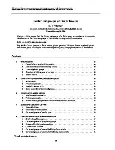
Consider the functions g0 and g1 specified by their sets of breaks as follows:         1 5 5 3 7 7 3 3 , , , , , , , g0 has breaks 8 8 2 8 8 4 8 8         3 3 7 1 1 9 5 5 g1 has breaks , , , , , , , 8 8 16 2 2 16 8 8 These functions have graphs as below.

10

g0

g1

Lemma 5.1 Let g0 and g1 be the functions in F that are defined above. Then hg0 , g1 i 1. consists of every element of F whose support is contained in the interval [ 38 , 78 ], and 2. is isomorphic with F . Proof: We only need show the first point. The second point will then follow since by Lemma 4.4 in [6] the subset of elements of F with support in [a, b] where a and b are diadic rationals with b − a an integral power of two is conjugate by a linear homeomorphism of R to produce exactly F . We explicitly build the linear conjugator of Lemma 4.4 in [6].
. This Consider the homeomorphism ω : R → R defined by t 7→ 8t−3 4 homeomorphism sends [ 83 , 78 ] linearly to [0, 1], and it induces an isomorphism ψ : hg0 , g1 i → H for some subgroup H ≤ Homeo(R). (Here, we are considering elements of F to be homeomorphisms from R to R, by using the unique extension of any element of F by the identity map away from [0, 1]). The function ψ can be thought of as a restriction of the inner automorphism of Homeo(R) produced by conjugation by ω. From here out, we will refer to hg0 , g1 i as Γ. If we restrict ψ less (potentially, depending on the size of Γ), and take the preimage of F under ψ −1 , then Lemma 4.4 in [6] tells us that ψ −1 (F ) = Υ∼ = F , where Υ consists of all graphs of F with support in [3/8, 7/8]. Since ω is linear, we can understand ψ by considering how the map ω moves the breaks of any element in hg0 , g1 i. If (pi , qi ), 1 ≤ i ≤ n, are the breaks of g ∈ hg0 , g1 i, then gψ is the unique piecewise-linear element of Homeo(R) whose breaks are ( 8pi4−3 , 8qi4−3 ) which acts as the identity near ±∞. 11

Now, one can check directly that g0 ψ = f0 and g1 ψ = f02 f1−1 f0−1 . So hg0 ψ, g1 ψi = hf0 , f02 f1−1 f0−1 i = hf0 , f0−2 (f02 f1−1 f0−1 )f0 i = hf0 , f1−1 i = hf0 , f1 i = F . In particular, ψ(Γ) = F , hence Υ = Γ, and Γ ∼ = F. ⋄

g0 ψ

g1 ψ

We are now ready to prove the first of our main theorems. For the following, we need to recall the K(a,b) groups: n o K(a,b) = h ∈ F | ∃m, n ∈ Z s.t. h′ (0) = (2a )n and h′ (1) = (2b )m

where both a and b are non-zero integers.

Theorem 1.1 Let H be a finite index subgroup of F . H is isomorphic to F if and only if H = K(a,b) for some a, b ∈ N . Proof: (⇐=): Fix a and b in N . We will build generators y0 and y1 for for K(a,b) . First, we will define y0 ∈ K(a,b) over a finite collection of points as follows: 1 1 1 , 8 ). If a 6= 1, then let (a1 , b1 ) = ( 22a , 21a ). If a = 1, then let (a1 , b1 ) = ( 16 Let (a2 , b2 ) = ( 18 , 38 ). Let (a3 , b3 ) = ( 85 , 78 ). If b = 1, then let (a4 , b4 ) = 1 1 ( 78 , 15 16 ). If b 6= 1, then let (a4 , b4 ) = (1 − 2b , 1 − 22b ). Filling in the definition of y0 . Extend the definition of y0 by making it linear from (0, 0) to (a1 , b1 ), affine and with slope one from (a2 , b2 ) to (a3 , b3 ), and affine from (a4 , b4 ) to (1, 1). All slopes involved so far are integral powers of two, and the set os ai ’s and bi ’s are all diadic rationals, so y0 still has the potential to be extended to an element of F . We can now pick some diadic rational pairs (c1 , d1 ) and (c2 , d2 ) with a1 < c1 < c2 < a2 and b1 < d1 < d2 < b2 so that the ratios d1 − b1 c1 − a1

and 12

b2 − d2 a2 − c2

both produce integral powers of 2 (not equal to the values of the slope of y0 near zero, or to the value 1, the slope of y0 over (a2 , a3 )), and where the line segments from (a1 , b1 ) to (c1 , d1 ) and from (c2 , d2 ) to (a2 , b2 ) (which we will be adding to the definition of y0 ) do not cross the line y = x. We can now extend the definition of y0 from 0 to c1 and from c2 to a3 so that over each interval, y0 admits precisely one breakpoint (over a1 and a2 respectively), and the graph of y0 determined so far stays well above the line y = x. By Lemma 3.5, there is an element ζ of F which sends the list of points (0, a1 , c1 , c2 , a2 , a3 , a4 , 1) to the list (0, b1 , d1 , d2 , b2 , b3 , b4 , 1). Assume we have previously expanded these lists as necessary with many diadic points imbetween c1 and c2 and correspondingly many diadic points between d1 and d2 , (all new points roughly evenly spaced out) so that the graph of ζ cannot intersect the line y = x. We can now define y0 over the interval (c1 , c2 ) to agree with ζ. The element y0 is now defined over the intervals (0, a3 ) and (a4 , 1). We can fill in the definition of y0 with similar care over the region (a3 , a4 ) (choose diadics c3 and c4 with a3 < c3 < c4 < a4 in a fashion similar to our choices of c1 and c2 , then connect over the region (c3 , c4 ) by some random appropriate element of F which does not touch the line y = x) to finally get an element y0 in F which 1. is linear over (0, a1 ), (a2 , a3 ), and (a4 , 1), and 2. has breakpoints including (a1 , b1 ), (a2 , b2 ), (a3 , b3 ), and (a4 , b4 ), and 3. does not intersect the line y = x. Note that while y0 is defined everywhere, it is not completely determined over (c1 , c2 ), and it is not completely determined over the similar interval (c3 , c4 ) in (a3 , a4 ) (although it is roughly controlled in both locations). Construct y1 as follows:

ty1 =

 

t : t ≤ 3/8 2t − (3/8) : 3/8 ≤ t ≤ 5/8  : 5/8 ≤ t ≤ 1 ty0

sub-claim 1.1.1: K(a,b) E F .

Proof of 1.1.1: Let g, h ∈ K(a,b) . Suppose g′ (0) = (2a )m and h′ (0) = Since all elements of F are linear in a neighborhood of 0, then the chain rule for derivatives from the right applies. In particular (gh)′ (0) = (2a )n .

13

(2a )m+n . Similarly, (gh)′ (1) = (2b )p+q , where g′ (1) = (2b )p and h′ (1) = (2b )q . So K(a,b) is a subgroup of F . Let f ∈ F . From Lemma 3.3, it must be the case that (gf )′ (0) = (2a )m and (gf )′ (1) = (2b )p . So gf ∈ K(a,b) . Thus K(a,b) E F . sub-claim 1.1.2: K(a,b) is a finite index subgroup of F. Proof of 1.1.2: Let f ∈ F . The slope of f near 0 is 2p and the slopes of elements of K(a,b) near 0 is 2an for n ∈ Z. Then the slopes of elements of f K(a,b) near 0 is 2an+p . The division algorithm gives us that since n ∈ Z, there are exactly a different cosets of K(a,1) . Similarly, there are exactly b different cosets for K(1,b) . Since K(a,b) = K(a,1) ∩ K(1,b) , then are at most ab distinct cosets for K(a,b) in F . sub-claim 1.1.3: Y = hy0 , y1 i ∼ = F. Proof of 1.1.3: y0 and y1 have been constructed specifically to have orbitals of certain products of these functions to be disjoint. Since y0 |[ 5 ,1] = 8 y1 |[ 5 ,1] , and as both functions have graphs above the line y = x in this 8

region, it must be the case that Supp(y0 y1−1 ) = (0, 58 ). By Lemma 3.3, y2

Supp(y1y0 ) = ( 58 , 1) and Supp(y1 0 ) = ( 87 , 1). By Lemma 3.1, [y0 y1−1 , y1y0 ] = 1 y2

and [y0 y1−1 , y1 0 ] = 1. y0 and y1 do not commute because 14 y0 y1 y0−1 y1−1 = −1 −1 5 −1 −1 3 −1 3 1 1 ∼ 2 y1 y0 y1 = 8 y0 y1 = 8 y1 = 8 6= 4 . So then by Lemma 3.6, Y = F . sub-claim 1.1.4: Y = hy0 , y1 i = K(a,b) . Proof of 1.1.4: Note that y1′ (0) = 1, y1′ (1) = y0′ (1), ( (1/8) ( (1/16) −1 if b = 1 1 if a = 1 (1/8) = 2 (1/16) = 2 ′ ′ y0 (0) = (1) = and y . a 0 (1/2 ) (1/22b ) −b if b > 1 = 2a if a > 1 = 2 b (1/22a ) (1/2 ) So y0 and y1 are both in K(a,b) and Y = hy0 , y1 i ⊆ K(a,b) . We have carefully constructed y0 and y1 in such a way that even though there are two intervals over which y0 is not explicitly known, the commutator function [y0 , y1 ] is completely determined. Let us demonstrate this point. Since y0 |[5/8,1] = y1 |[5/8,1] , then y0 y1 y0−1 y1−1 |[5/8,1] = 1. Since y1 |[0,3/8] = 1 and 18 y0 = 38 , then y0 y1 y0−1 y1−1 |[0,1/8] = 1. The following line segments are taken linearly to each other.           1 1 y0 3 1 y1 3 5 y0−1 1 3 y1−1 1 3 7−→ 7−→ , , , 7−→ , 7−→ , . 8 4 8 2 8 8 8 8 8 8 14



         1 3 y0 1 5 y1 5 7 y0−1 3 5 y1−1 3 1 , , , , , 7 → − 7−→ 7−→ 7−→ . 4 8 2 8 8 8 8 8 8 2     3 5 y0 5 7 , , 7−→ 8 8 8 8     Since y1 y0−1 |[5/8,1] = 1, then y0 y1 y0−1 linearly maps 38 , 58 to 85 , 78 , which is taken linearly by y1−1 to [ 12 , 58 ]. Now y0 y1 y0−1 y1−1 contains the straight line segments from (0, 0) to ( 18 , 18 ), from ( 18 , 18 ) to ( 14 , 38 ), from ( 14 , 83 ) to ( 38 , 12 ), from ( 38 , 12 ) to ( 85 , 58 ), and from ( 58 , 58 ) to (1, 1). Since Supp([y0 , y1 ]) = ( 18 , 58 ) and y0 is explicitely known in the interval 1 5 ( 8 , 8 ), then we can explicitely find [y0 , y1 ]y0 . Also, since Supp([y0 , y1 ]y0 ) = −1 ( 38 , 78 ) and y1−1 is explicitely known on ( 83 , 78 ), then [y0 , y1 ]y0 y1 can also be −1 computed. This computation gives that [y0 , y1 ]y0 = g0 and [y0 , y1 ]y0 y1 = g1 , where g0 and g1 are the functions defined in the beginning of Section 5. So then by Lemma 5.1, hg0 , g1 i contains every element of F that has support inside the interval ( 38 , 78 ). Since g0 and g1 are products of the funtions y0 , y1 ∈ K(a,b) , then Y and K(a,b) both contain every element of F whose support is contained in the interval ( 83 , 87 ). Let h ∈ F ′ . By Lemma 3.7, there exists a c, d ∈ (0, 1) so that Supp(h) ⊆ (c, d). By Lemma 3.4, since Supp(y0 ) = (0, 1), there is an n ∈ Z so that n Supp(hy0 ) ⊆ ( 38 , dy0n ), where 38 < cy0n < dy0n < 1. By Lemma 3.4, since Supp(y1 ) = ( 38 , 1), then there is an m ∈ Z so that 38 = 83 y1m < cy0n y1m < m n dy0n y1m < 78 and Supp((hy0 )y1 ) ⊆ ( 83 , 78 ). By the previous argument, it must −m −n n m n m be the case that hy0 y1 ∈ Y . So then h = (hy0 y1 )y1 y0 ∈ Y . So F ′ ⊆ Y . Let w ∈ K(a,b) . There is an n, m ∈ Z so that w′ (0) = 2an and w′ (1) = 2bm . Since w, y0 , and y1 are all linear functions in a neighborhoods of 0 and 1, then the chain rule gives (wy0−n )′ (0) = (2an )(2a )−n = 1, (wy0−n )′ (1) = (2bm )(2−b )−n = 2b(m+n) , (wy0−n y1m+n )′ (0) = (1)(1)m+n = 1, and (wy0−n y1m+n )′ (1) = 2b(m+n) (2−b )m+n = 1. So wy0−n y1m+n ∈ F ′ ⊆ Y ⇒ w ∈ Y . Thus K(a,b) = Y ∼ = F. (=⇒): Assume that H is a finite index subgroup of F and H ∼ = F. By Lemma 1.4, H E F . By Lemma 1.3, F ′ ≤ H so Supp(H) = (0, 1). There exists functions h0 and h1 so that H = hh0 , h1 i that satisfy the conditions listed in Lemma 3.8. One condition in Lemma 3.8 is if A is an orbital of h0 and B is an orbital of h1 , then either B ⊆ A or B ∩ A = ∅. This guarantees that if p is a fixed point of h0 , then p is also a fixed point 15

of h1 . So then the point p will be a fixed point of the group H. So p ∈ / supp(H) = (0, 1). So either p = 0 or p = 1 and Supp(h0 ) = (0, 1). Since h0 is not the identity near either 0 or 1, then there exist nonzero integers a and b so that h′0 (0) = 2a and h′0 (1) = 2b . Lemma 3.8 also guarantees that either h′1 (0) = 1 and h′1 (1) = 2b or h′1 (0) = 2a and h′1 (1) = 1. Without loss of generality, assume h′1 (0) = 1 and h′1 (1) = 2b . We want to show that H = K(a,b) . (⊆) : h0 ∈ K(a,b) and h1 ∈ K(a,b) , so H = hh0 , h1 i ⊆ K(a,b) . (⊇) : Let f ∈ K(a,b) . So f ′ (0) = 2an and f ′ (1) = 2bm for some ′ an a −n = 1 and n, m ∈ Z. Then, by the chain rule, (f h−n 0 ) (0) = (2 )(2 ) −n ′ −n n−m ′ bm b −n b(m−n) (f h0 ) (1) = (2 )(2 ) =2 . Also, (f h0 h1 ) (1) = 1(1)n−m = −n n−m ′ b(m−n) b 1 and (f h0 h1 ) (1) = 2 (2 )n−m = 1. So then by Lemma 3.7, n−m n−m f h−n ∈ F ′ . Since H E F , then F ′ ⊆ H. So f h−n ∈ H. So then 0 h1 0 h1 −n n−m m−n n f = f h0 h1 h1 h0 ∈ H. So H = K(a,b) . ⋄ Theorem 1.2 Given any positive integers a and b, F can be regarded as a non-split extension of Za × Zb by F . In particular, there are maps ι and τ so that the following sequence is exact. 1

/F

ι

/F

τ

/ Za × Zb

/ 1.

Proof : This theorem is actually an immediate corollary to Theorem 1.1; simply take ι to be the composition of the isomorphism from F to K(a,b) with the inclusion map of K(a,b) into F . ⋄ To prove Theorem 1.6, we will need to produce some analysis of the finite index subgroups of Z 2 .

6

Finite index subgroups of Z 2

In this section we will prove two statements about the finite index subgroups of Z 2 . While both of these statements could be taken as straightforward exercises in an entry level graduate course in group theory, we will include the proofs for completeness. Lemma 6.1 Suppose H is a finite index subgroup of Z 2 . Then there are ˜ (a,b) ≤ H. Further, if K ˜ (c,d) ≤ H minimal positive integers a and b so that K ˜ (c,d) ≤ K ˜ (a,b) . then K 16

Proof: H is normal in Z 2 since Z 2 is abelian. In particular, since H has finite index in Z 2 , the group T = Z 2 /H is finite. Therefore, there is a minimal positve integer a so that (a, 0) ∈ H and a minimal positive integer b so that ˜ (a,b) ≤ H. (0, b) ∈ H. It is now immediate that K ˜ Suppose K(c,d) ∈ H. Then (c, 0) ∈ H. The Euclidean Algorithm now shows that (j, 0) ∈ H, where j = gcd(a, c). If a ∤ c we must have that j < a, which contradicts our choice of a. In particular, a | c and (c, 0) ∈ ˜ (a,b) . A similar argument shows that (0, d) ∈ K ˜ (a,b) . Since K ˜ (c,d) h(a, 0)i ≤ K ˜ ˜ is generated by (c, 0) and (0, d), we have that K(c,d) ≤ K(a,b) . ⋄ ˜ (a,b) the maximal K ˜ group In the above lemma, we will call the group K in H. ˜ Lemma 6.2 Suppose H is a finite index subgroup in Z 2 with maximal K ∼ ˜ ˜ group K(a,b) . The group Q = H/K(a,b) is finite cyclic. ˜ (a,b) Proof: Thinking of Z 2 as a planar lattice, the points in H not in K ˜ (a,b) to become are the points which will survive under modding H out by K non-trivial elements of Q. Thus, we can find Q as a subgroup of points in the finite rectangular lattice L = Za × Zb . Furthermore, as a and b are minimal positive so that (a, 0) ∈ H and (0, b) ∈ H, we must have that the only intersection Q will have with the vertical axis in L (the points of the form (0, r)) or with the horizontal axis in L (the points of the form (r, 0)) is at the point (0, 0). In particular, suppose (r, s) and (t, u) are points in Q. If j ≡ gcd(r, t), then we can again exploit the Euclidean Algorithm to find integers p and q so that p(r, s)+q(t, u) = (j, m) so that j divides both r and t. In Za ×Zb the point (j, m) ∈ Z 2 becomes (j, mb ). Now there are positive integers x and y so that x(j, mb ) = (r, xmb ) and y(j, mb ) = (t, ymb ). If xmb 6≡ s mod b then Q has an intersection with the vertical axis in Za × Zb away from (0, 0) and if ymb 6≡ u mod b then Q has an intersection with the vertical axis of Za × Zb away from (0, 0). Since neither of these intersections can exist, by the definitions of a and b, we see that (r, s) and (t, u) ∈ h(j, mb )i in Q. In particular, after a finite induction we see that Q is cyclic. ⋄

7

The structure of the extension

We have now done enough work so that Theorem 1.6 is transparent. 17

Theorem 1.6 1. The map φ induces a one-one correspondence between the finite index subgroups of F and the finite index subgroups of Z 2 . ˜ = φ(H) ≤ 2. Let H be a finite index subgroup H of F , with image H Z × Z. There exist smallest positive integers a and b with K(a,b) ≤ H. ˜ K ˜ (a,b) , then Q is finite cyclic, and there are Furthermore, if Q = H/ maps ι, ρ, ˜ι and ρ˜ so that the diagram below commutes with the two rows being exact: F ∼ =

1

 /K

ι

φ|K

ρ

/Q

/1

/Q

/ 1.

φ|H



1

/H

/K ˜

˜ ι

 /H ˜

ρ˜

Proof: The first point follows from Lemma 1.3 and the fact that the kernel of φ is F ′ . The second point follows from a conglomeration of lemmas. The existence of minimal positive integers a and b (so that K(a,b) is ˜ (a,b) in H, ˜ which maximal in H) follows from the existence of a maximal K is lemma 6.1. The fact that Q is finite cyclic comes from Lemma 6.2. The isomorphism from F to K = K(a,b) comes from Theorem 1.1. The map ι is the inclusion map of K(a,b) into H. The map ˜ι is induced from the projection φ. the map ρ˜ is the natural quotient onto Q of the image ˜ The bottom row is thus exact. ρ is the composition of the natural of ˜ι in H. quotient of H by the image of ι followed by the isomorphism from H/ι(K) ˜ ι(K) ˜ = Q, thus, the top row is exact, and the diagram commutes. to H/˜ ⋄ To prove Lemma 1.7 we will make use of Rubin’s Theorem. The version we will quote is Theorem 2 in Brin’s paper [3]. That version is itself derived from Theorem 3.1 in the paper [8] of Rubin, where in the statement of the theorem, a technical hypothesis is inadvertently missing (see the discussion of this in [3]). In order to state Rubin’s Theorem, we will need to define some terminology. In this, we generalize the language of the definition of locally 18

dense given in Brin’s [3]. Our generalization will have no impact on the content of our statement of Rubin’s theorem. Suppose X is a topological space and H(X) is its full group of homeomorphisms. Suppose further that K ≤ H(X). Given W ⊂ X, we will say K acts locally densely over W if for every w ∈ W and every open U ⊂ W with w ∈ U , the closure of  wκ|κ ∈ K, κ|(W −U ) = 1(W −U )

contains some open set in W . In particular, for each open U in Z, the subgroup of elements fixed away from U has every orbit in U dense in some open set of W in U . We are now ready to state Rubin’s theorem. We give essentially the statement given in [3], although we recast it in the language of right actions. Theorem 7.1 (Rubin) Let X and Y be locally compact, Hausdorff topological spaces without isolated points, Let H(X) and H(Y ) be the self homeomorphism groups of X and Y , respectively, and let G ⊆ H(X) and H ⊆ H(Y ) be subgroups. If G and H are isomorphic and both act locally densely over X and Y , respectively, then for each isomorphism ϕ : G → H there is a unique homeomorphism γ : X → Y so that for each g ∈ G, we have gϕ = γ −1 gγ. In our case, and to apply Rubin’s theorem to F or subgroups of F , we need to consider these groups to be groups of homeomorphisms of (0, 1), instead of [0, 1]. This comes from the simple fact that F does not move 0 or 1 to produce a dense image in any open set! Having made that (temporary) change to our definition of F and its subgroups, we are ready to apply Rubin’s theorem to any such subgroup, as long as it is locally dense in its action on (0, 1). In the discussion which follows, given X ⊂ R, we will use the notation DX to denote the set Z[1/2] ∩ X of diadic rationals in X. Lemma 7.2 Finite index subgroups of F act locally densely on (0, 1). Proof: Suppose H is finite index in F , and x ∈ (0, 1) and U an open neighborhood of x in (0, 1). Let d1 and d2 be two diadic rationals in U with d1 < x < d2 . let K be the subgroup of F consisting of all the elements of F with support in (d1 , d2 ). Let α : R → R be any piecewise-linear homeomorphism which is the identity near ±∞ and which has all slopes integral powers of 2, and with all breaks occuring over the diadic rationals, and that 19

maps d1 to 0 and d2 to 1. It is easy to build such a map, and the reader may check that the inner automorphism of Homeo(R) generated by conjugation by α will take K isomorphically to F . Now by an induction argument (for instance, as carried out in the first paragraph of Section §1. in [6]), it is easy to see that α takes D(d1 ,d2 ) to D(0,1) in an order preserving fashion. In particular, as F is k-transitive on D(0,1) for any positive integer k (recall Lemma 3.5), we see that K is k-transitive on D(d1 ,d2 ) for any positive integer k. Now, if x is a diadic rational, then the orbit of x under K is dense in (d1 , d2 ), as K acts transitively over D(d1 ,d2 ) , and D(d1 ,d2 ) is dense in (d1 , d2 ). If x is not diadic rational, then given any ǫ > 0, and any y in (d1 , d2 ), we can find four diadic rationals x1 ,x2 , y1 , y2 ∈ (d1 , d2 ) so that x1 < x < x2 and y1 < y < y2 , and where the yi are chosen epsilon-close to y. Now there is some element κ in K which throws x1 to y1 and x2 to y2 (since K is 2-transitive over D(d1 ,d2 ) ). In particular, |y − xκ| < ǫ. Hence, the orbit of x is dense in (d1 , d2 ). Now, as K ≤ F ′ ≤ H, H is locally dense over (0, 1). ⋄ We will use Rubin’s theorem to prove the final lemma from the introduction. Lemma 1.7 Suppose H, H ′ ∈ F IF , K = Inner(H), K ′ = Inner(H ′ ), and ξ : H → H ′ is an isomorphism. Then 1. ξ(K) = K ′ 2. K is characteristic in H and K ′ is characteristic in H ′ , and 3. Res(H) = Res(H ′ ). Proof: First, let us suppose ϑ : H → H ′ is an isomorphism. By Lemma 7.2, H and H ′ both act locally densely on (0, 1). In particular, Rubin’s theorem tells us that there is a homeomorphism γ : (0, 1) → (0, 1) so that for any h ∈ H, ϑ(h) = γ −1 hγ ∈ H ′ . Now by Lemma 3.3, we see that the collection of orbitals of h′ = ϑ(h) is in bijective correspondence with the orbitals of h. Further, if γ is orientation-preserving, any orbital of h which has end e ∈ {0, 1} becomes (under the action of γ) an orbital of h′ with end e. If γ is orientation-reversing, then any orbital of h with end e ∈ {0, 1} becomes an orbital of h′ with end f 6= e, where f ∈ {0, 1}. 20

Since ϑ is a homomorphism, a consequence of the above paragraph is if K = K(a,b) for some positive integers a and b, then there are positive integers c and d with ϑ(K) = K(c,d) ≤ K ′ ≤ H ′ . The correspondence theorem now tells us that the maximal rectangular groups of H and H ′ are mapped precisely to each other by ϑ, and we have point (1). The second two points follow immediately. Note that this argument provides a second proof that amongst the finite index subgroups of F , only the rectangular groups are actually isomorphic to F . ⋄ The lemma above provides the key ingredients for the proof of our final theorem. Recall the isomorphisms τ(a,b) : K(a,b) → F from the introduction (elements of K(a,b) with slope (2a )s near zero are taken to elements of F with slope 2s near zero, and elements of F with slope (2b )t near one are taken to elements of F with slope 2t near one), and the map Outer which, given a finite index subgroup H of F , produces the smallest rectangular subgroup of F that contains H. With these maps in mind, and with the above lemma in hand, we are finally ready to prove our last theorem. Theorem 1.8: Suppose H, H ′ are finite index subgroups of F . Let a, b, c, d be positive integers so that K(a,b) = Outer(H), K(c,d) = Outer(H ′ ). H is isomorphic with H ′ if and only if τ(a,b) (H) = τ(c,d) (H ′ ) or τ(a,b) (H) = Rev(τ(c,d) (H ′ )). Proof: Suppose that ϑ : H → H ′ is an isomorphism. Lemma 1.7 assures us that there is a well defined positive integer n so that Res(H) = Res(H ′ ) = n, and ϑ(K) = K ′ . Let us further suppose that K(r,s) = Inner(H) and K(t,u) = Inner(H ′ ). ˜ = φ(H), and H ˜ ′ = φ(H ′ ). Consider the translations of Z 2 genLet H ˜ is a group, the sets H, ˜ H ˜ + (r, 0), and erated by (r, 0) and (0, s). Since H ˜ H + (0, s) are the same. In particular, we can consider the image in the lat˜ restricting our view to the rectangle R of points with integer tice Z 2 of H, coordinates where the horizontal coordinates range from 0 to r − 1 and the vertical coordinates range from 0 to s − 1, and understand everything about ˜ K ˜ (r,s) only intersects R at (0, 0), while there are n total interthe group H. ˜ sections of H with R, all obtained by translating different powers of some particular vector (p, q) into R (using (r, 0) and (0, s)). Let j = gcd(p, r). So, the lowest column number that the image of the translated powers of 21

˜ intersects R exactly n times, (p, q) in R will appear in is column j. Since H it must be that case that nj = r and the images of the translated powers of (p, q) in R will occur in columns 0, r/n, 2r/n, ... ,(n − 1)r/n. Similarly, gcd(q, s) = s/n and the images of the translated powers of (p, q) in R will ˜ (a,b) is the smallest occur in rows 0, s/n, 2s/n, ... ,(n − 1)s/n. Now, as K ˜ rectangular group to contain H, we see that a = r/n and b = s/n. A similar discussion shows that c = t/n and d = u/n. Stated another way, we have r s t u = = = = n. a b c d Now, consider the image of H and H ′ under the respective maps τ(a,b) and τ(c,d) . The subgroups K(r,s) = Inner(H) and K(t,u) = Inner(H ′ ) are both taken to K(n,n) . We will now assume that this is how H and H ′ started out, and do all remaining work in these scaled versions of H and H ′ . The isomorphism ϑ which is carrying H to H ′ must now preserve the maximal rectangular subgroup K(n,n) , by Lemma 1.7. By Lemma 7.2, both H and H ′ act locally densely on (0, 1), so by Rubin’s theorem there is a homeomorphism γ so that for any h ∈ H, ϑ(h) = γ −1 hγ ∈ H ′ . Note that as γ need not be piecewise-linear, we should be concerned that conjugating by γ might change slopes, as well as potentially swapping coordinates. By Lemma 1.7 we know that K(n,n) = Inner(H) = Inner(H ′ ) is being brought isomorphically to itself by ϑ. Suppose h ∈ H has an orbital A. Denote by EA the set of ends of A which are in the set {0, 1}. Now consider h′ = ϑ(h). The element h′ has an orbital B = γ(A) by point (1) of Lemma 3.3. Denote by EB the ends of B that are actually in the set {0, 1}. Then as γ preserves the set {0, 1} we see that the cardinalities of EA and EB must be the same. Now, by the result of the previous paragraph, and using the fact that the ϑ takes K(n,n) isomorphically to itself, we see that if γ is orientationpreserving, we must have that γ will send (n, 0) to (n, 0) and (0, n) to (0, n) in the induced map from φ(H) → φ(H ′ ) (note that (n, 0) will not be taken to (−n, 0), as conjugation by an orientation-preserving γ will preserve the local directions that points near zero and one move under the action of h). Similarly, if γ is orientation-reversing, then the reader can check that the action of γ will send (n, 0) to (0, n) and (0, n) to (n, 0), again considering the induced map from φ(H) → φ(H ′ ). If γ is orientation-reversing, then replace H ′ by the isomorphic copy Rev(H ′ ), so that from here out we only need to argue the case where our

22

isomorphism ϑ appears to be the identity after passing through the quotient map φ. Suppose f ∈ H. φ(f ) = (v, w), if and only if φ(ϑ(f )) = (v, w). But now as H and H ′ both contain the commutator subgroup F ′ , and as they each contain an element which has slopes 2v and 2w near zero and one respectively, we see that both H and H ′ contain all of the elements of F with φ(k) = (v, w). It is now immediate that H = H ′ . Now let us suppose that H and H ′ are finite index subgroups of F , and that K(a,b) = Outer(H) and K(c,d) = Outer(H ′ ). Let us further suppose that the scaling maps τ(a,b) and τ(c,d) have the property that τ (a, b)(H) = τ (c, d)(H ′ ) or τ(a,b) (H) = Rev(τ (c, d)(H ′ )). Since the τ(∗,∗) maps are isomorphisms, and the map Rev is an isomophism, we immediately see that H and H ′ are isomorphic. ⋄

8

Some examples

In this section, we give some examples of finite index subgroups of F , and consider them from the perspective of this paper. Example 1: Let H = {f ∈ F | f ′ (0) = 23n+5m and f ′ (1) = 27n+11m for some m, n ∈ Z}. H is a finite index subgroup of F but H is not isomorphic to F . ˜ = φ(H). Since 3, 5, 7, and 11 are all odd, the only possible Let H ˜ are (even, even) and (odd, odd). If n = 5 and m = −3, elements of H ˜ If n = −11 and m = 7, then (−33 + then (15 − 15, 35 − 33) = (0, 2) ∈ H. ˜ ˜ If n = −3 35, −77 + 77) = (2, 0) ∈ H. So then every (even, even) is in H. ˜ Since (1, 1) and all (even, even) are in H, ˜ then and m = 2, then (1, 1) ∈ H. ˜ ˜ all (odd, odd) are also in H. So H is index 2 in Z ⊕ Z and H is index 2 in F. To show that H is not isomorphic to F , it is enough to show that H 6= K(a,b) for any non-zero integers a and b. Assume that for some non-zero integers a and b, H = K(a,b) . If h ∈ H, there are integers p and q such that φ(h) = (ap, bq). There is an f ∈ H so that φ(f ) = (3, 7). There is a g ∈ H so that φ(g) = (5, 11). Now, there must be integers p1 and p2 so that ap1 = 3 and ap2 = 5. Thus a = 1. Also, there must be integers q1 and q2 so that bq1 = 7 and bq2 = 11. So b = 1. But K(1,1) = F 6= H, so H can not be isomorphic to F . ⋄ ˜ (a,b) group was K ˜ (2,2) , In the above example, note that the maximal K 23

˜ and that the quotient H/ ˜ K ˜ (2,2) ∼ which was proper in H, = Z2 . In particular, H is isomorphic to a non-split extension of F by Z2 , where the structure of ˜ as an extension of K ˜ (2,2) by the extension is described by the structure of H Z2 . Example 2: Let l,r,f , f ′ ∈ F , so that φ(l) = (15, 0), φ(r) = (0, 15), φ(f ) = (3, 3), and φ(f ′ ) = (3, 6). Suppose that H = hF ′ , l, r, f i while H ′ = hF ′ , l, r, f ′ i. We see immediately that the maximal rectangular subgroups of H and ′ H are K(15,15) . The minimal rectangular subgroups of F containing H and H ′ are the same, namely K(3,3) . The residues of H and H ′ are both 5, but H and H ′ are not isomorphic, as τ(3,3) (H) 6= τ(3,3) (H ′ ) and τ(3,3) (H) 6= Rev(τ(3,3) (H ′ )). Below is included a diagram of the rectangle R in Z 2 which demonstrates this non-equality.

4

3

H 2

H’ 1

0

0

1

2

3

4

Example 3: Let l1 , l2 , r1 and r2 ∈ F so that φ(l1 ) = (10, 0), φ(l2 ) = (35, 0), φ(r1 ) = (0, 15), and φ(r2 ) = (0, 20). Further, let g1 , g2 ∈ F so that φ(g1 ) = (2, 6) and φ(g2 ) = (14, 4). Let H = hF ′ , l1 , r1 , g1 i and let H ′ = hF ′ , l2 , r2 , g2 i. It is immediate that Inner H = K(10,15) , Outer H = K(2,3) , Inner H ′ = K(35,20) , and Outer H ′ = K(7,4) . Both H and H ′ have residue 5. If we apply τ(2,3) to Outer H and τ(7,4) to Outer H ′ , and draw our fundamental 5 × 5 rectangle in Z 2 , we get the following diagram. (Below, we are considering H and H ′ after the rescaling.)

24

4

3

H 2

H’ 1

0

0

1

2

3

4

The scaled version of H is Rev of the scaled version of H ′ , so that H∼ = H ′.

25

References [1] Collin Bleak, A geometric classification of some solvable groups of homeomorphisms, preprint (2006), 1–26. [2] Matthew G. Brin, The ubiquity of Thompson’s group F in groups of piecewise linear homeomorphisms of the unit interval, J. London Math. Soc. (2) 60 (1999), no. 2, 449–460. [3]

, Higher dimensional Thompson groups, Geom. Dedicata 108 (2004), 163–192.

[4] Matthew G. Brin and Craig C. Squier, Groups of piecewise linear homeomorphisms of the real line, Invent. Math. 79 (1985), no. 3, 485–498. [5] Jos´e Burillo, Sean Cleary, and Claas R¨ over, Commensurations and Subgroups of Finite Index of Thompson’s Group F, arXiv:0711.0919 (2007), 1–12. [6] J. W. Cannon, W. J. Floyd, and W. R. Parry, Introductory notes on Richard Thompson’s groups, Enseign. Math. (2) 42 (1996), no. 3-4, 215– 256. [7] Sean Cleary and Jennifer Taback, Thompson’s group at forty years, AIM Workshop (preliminary problem list) (2004), 1–11. [8] Matatyahu Rubin, Locally moving groups and reconstruction problems, Ordered Groups and permutation groups (1996), 121–157. [9] Bronlyn Wassink, Subgroups of R. Thompson’s group F, Dissertation, Binghamton University, New York, 2007, In Preparation.

26