Firefly-inspired Heartbeat Synchronization in Overlay Networks∗
Ozalp Babaoglu Univ. Bologna, Italy
[email protected]
Toni Binci Univ. Bologna, Italy
[email protected]
M´ark Jelasity HAS & Univ. Szeged, Hungary
[email protected]
Alberto Montresor Univ. Trento, Italy
[email protected]
Abstract Heartbeat synchronization strives to have nodes in a distributed system generate periodic, local “heartbeat” events approximately at the same time. Many useful distributed protocols rely on the existence of such heartbeats for driving their cycle-based execution. Yet, solving the problem in environments where nodes are unreliable and messages are subject to delays and failures is non-trivial. We present a heartbeat synchronization protocol for overlay networks inspired by mathematical models of flash synchronization in certain species of fireflies. In our protocol, nodes send flash messages to their neighbors when a local heartbeat triggers. They adjust the phase of their next heartbeat based on incoming flash messages using an algorithm inspired by mathematical models of firefly synchronization. We report simulation results of the protocol in various realistic failure scenarios typical in overlay networks and show that synchronization emerges even when messages can have significant delay subject to large jitter.
1. Introduction In cycle- or round-based distributed protocols (such as gossip protocols), it is often necessary that all nodes agree on when a new cycle starts. In other words, the local perceptions at nodes as to when cycles begin and end ∗ Authors
are listed in alphabetical order. Partial support for this work was provided by the European Union within the 6th Framework Programme under contracts 001907 (DELIS) and 27748 (BIONETS).
need to be synchronized so that we can talk about “cycles” of the system as a whole. For example, if the protocol requires periodic restarts (that is, all nodes need to be re-initialized), it is important that this event be synchronized [7, 9]. Heartbeat synchronization strives to have nodes in a distributed system generate periodic, local “heartbeat” events approximately at the same time. It differs from classical clock synchronization in that nodes are not interested in counting cycles and agreeing on the ID of the current cycle. Furthermore, there is no requirement regarding the length of a cycle with respect to real time as long as the length is bounded and all nodes agree on it eventually. What we are interested in guaranteeing is that all nodes start and end their cycles at the same time, with an error that is at least one, but preferably more, orders of magnitude smaller than the chosen cycle length. This problem is rather difficult to solve in peer-topeer overlay networks due to dynamism, failures and scale. In overlay networks, message delay can vary over a wide range [10] and churn can be significant with nodes leaving and joining the network continuously. In addition, overlay networks can be extremely large, containing millions of nodes. This implies that any proposed solution must be highly scalable. And finally, the solution needs to be decentralized for it to be usable in overlay networks where nodes have only partial information regarding the system as a whole. Our approach to achieving robust, scalable and decentralized heartbeat synchronization is based on biological inspiration drawn from the flashing of fireflies. It is well know that in certain firefly species, male mem-
bers gather in large numbers at dusk and are able to synchronize their flashes such that eventually the entire swarm flashes in unison. What is surprising is that global synchronization emerges despite the fact that each member can observe only some small neighborhood of the swarm and can modifies its own flashing behavior based on this limited local information. Several mathematical models have been proposed to explain this phenomenon (see for example [13] and references therein). Decentralized synchronization protocols based on such models have been suggested before in the context of wireless sensor networks [16]. To our knowledge, mathematical models of firefly synchronization have not been applied to solve problems in large scale overlay networks. The main contribution of the paper is twofold. First, in Section 3 we introduce a novel protocol for heartbeat synchronization in overlay networks that is based on an adaptive mathematical model of emergent synchronization of firefly flashing [3]. Second, in Section 4 we present extensive large-scale event-based simulation studies of the protocol in realistic scenarios involving message loss and delay, and demonstrate that the protocol can indeed achieve synchronization to a sufficient degree.
2. System Model We assume that nodes are connected through an existing routed network, such as the Internet, where every node can potentially communicate with every other node. To actually communicate, a node has to know the address of another node. This is achieved by maintaining a partial view (view for short) at each node that contains a set of node descriptors. Views can be interpreted as sets of edges between nodes, naturally defining a directed graph over the nodes that determines the topology of an overlay network. The network is highly dynamic; new nodes may join at any time, and existing nodes may leave, either voluntarily or by crashing. Our approach does not require any mechanism specific to leaves: spontaneous crashes and voluntary leaves are treated uniformly. Thus, in the following, we limit our discussion to node crashes. Byzantine failures, with nodes behaving arbitrarily, are excluded from the present discussion. Communication incurs unpredictable delays and is subject to failures. Single messages may be lost, links between pairs of nodes may break. Nodes have access
1: 2: 3: 4: 5:
loop wait until φ = 1 P ← selectPeerList() send flash to all peers in P end loop (a) active thread
1: 2: 3: 4:
loop receive flash processFlash() end loop (b) passive thread
Figure 1. The skeleton of the heartbeat synchronization protocol. to local clocks that can measure the passage of real time with reasonable accuracy, that is, with small short-term drift.
3. The Synchronization Protocol In this section we present an abstract protocol skeleton for firefly-inspired heartbeat synchronization and overview some of its possible instantiations based on different mathematical models of firefly flashing behavior. We briefly discuss the behavior of each model and argue that the most promising one is the adaptive model described in [3]. This model will be analyzed experimentally in Section 4.
3.1. The Protocol Skeleton The protocol skeleton is shown in Figure 1. We assume that each node is an oscillator that can be characterized by its phase, φ , and the cycle length, ∆. The phase is a variable in the interval [0, 1] and its dynamics are defined by a sawtooth function of time t, where we have ∂ φ /∂ t = 1/∆, such that the phase increases linearly from 0 to 1 in ∆ time units. When the phase reaches 1, the node emits a “flash”, which results in a ping message being sent to a set of peer nodes. Subsequently, the phase is reset to 0. The cycle length ∆ can be initially different (or identical) at all nodes, depending on the implementation of PROCESS F LASH under consideration. When the node receives a flash, method PROCESS F LASH is executed. This method is the heart of the synchronization algorithm. It is responsible for updating φ and possibly also ∆. That is, it can delay or advance the
phase (and thereby the next flash), possibly as a function of the current phase, and it can adjust the cycle length as well. We will examine different implementations later in the section. Method SELECT P EER L IST relies on an underlying overlay network which is used to return a list of neighbors. In our experimental analyses, we will assume that this overlay network is random and dynamic with a small, constant number of neighbors for each node. As such, SELECT P EER L IST returns a small, random set of peer nodes. More details on the practical implementation of this random overlay will be given in Section 4. We now move on to describe three possible implementations of method PROCESS F LASH.
3.2. Phase-Advance and Phase-Delay The simplest possible implementation of PROCESS F LASH sets φ = 0 (phase-delay model) or φ = 1 (phaseadvance model). If we assume instant message delivery without failures, both choices result in the pairwise synchronization of the peers that sent and received the flash message. The only difference between the two choices is that in the case of phase-advance, a flash message is also emitted alongside the pairwise synchronization step. This model assumes that all nodes have exactly the same fixed cycle length ∆. Obviously, since the model does not involve the adjustment of the cycle length, if we start with heterogeneous values at the nodes, or if the skew of the clocks is significant, the model is not guaranteed to converge. Furthermore, the phase-advance model is highly impractical because of the cascading flash messages that are generated in the initial phase of the synchronization: advanced flash messages trigger more and more advanced flashes which quickly overloads the network. We note that if one can guarantee that the cycle lengths are indeed identical at all nodes, then the phase delay model performs rather well according to our preliminary experiments. However, due to lack of space, we do not pursue this model further in this paper, in order to be able to fully focus on the Ermentrout model described in Section 3.4.
3.3. The Mirollo-Strogatz Model The model of Mirollo and Strogatz [13] generalizes the simplistic phase-advance model in the following way. It introduces a third variable x, that we will call “voltage” to illustrate the intuition behind it. Voltage is defined by a non-linear function f : [0, 1] → [0, 1] as x = f (φ ), where f is smooth, monotone increasing, and concave down (in other words, the first two derivatives of f are continuous and satisfy f ′ > 0 and f ′′ < 0). The model also requires f (0) = 0 and f (1) = 1. The reason for introducing this nonlinearity through the new voltage variable is that it offers us an easy way to adjust the sensitivity of the phase adjustment depending on the actual phase. We advance the voltage by a fixed amount: x′ = min(x+ ε , 1) and set the phase to reflect the new voltage: φ ′ = f −1 (x′ ), where x′ and φ ′ is the new state after the update. If the phase is close to zero, then this update rule will change the phase relatively little, while towards the end of the cycle the node will become more and more sensitive to incoming flash messages. Note that if ε ≥ 1 then the model becomes identical to the phase-advance model. Theoretical results in [13] indicate that if the underlying overlay network is a clique (all nodes are connected to all other nodes), and messages are delivered instantly and without failures, then the model guarantees convergence. Recently, the assumption about full connectivity has been relaxed in [11]. Our preliminary experimental results confirm that, apart from flooding problems similar to the phaseadvance approach, the model is very sensitive to message delay and message loss.
3.4. The Adaptive Ermentrout Model In the model of Ermentrout, the nodes have a variable cycle length [3]. This model was motivated by the fact that fireflies indeed cannot have identical cycle lengths initially. In this model, the actual cycle length of node i becomes a variable δi which is bounded above and below: ∆l < δi < ∆u . In addition to the new global parameters ∆l and ∆u , each node has a parameter ∆ (∆l < ∆ < ∆u ) as well: its natural cycle length. A node will flash once in each ∆ time units in the lack of interaction with other nodes. The model is expressed in terms of the frequencies Ωl = 1/∆u , Ωu = 1/∆l , Ω = 1/∆ and ωi = 1/δi .
Previous implementations of PROCESS F LASH updated the phase variable φ thereby adjusting the time of the next flash. The interesting feature of the model of Ermentrout is that PROCESS F LASH updates the variable ω instead of variable φ . If a flash arrives “too late” (that is, when φ < 1/2), then the frequency is decreased (that is, cycle length is lengthened) while the phase remains unchanged. This increases the time until the next flash, so that it is more likely to be aligned with the next flash from the source of the received flash. Similarly, if the flash is “too early” (φ > 1/2), then the frequency is increased towards Ωu . According to [3], the update formula applied by PROCESS F LASH becomes
ω ′ = ω + ε (Ω − ω ) + g+(φ )(Ωl − ω ) + g−(φ )(Ωu − ω ) (1) where ω ′ is the new frequency, and the phase φ remains unchanged. The coefficients of the terms are ε , a parameter that controls the tendency of the frequency to move towards the common natural frequency Ω, and two functions g+ and g− defined as g+ (φ )
=
g− (φ )
=
sin 2πφ , 0) 2π sin 2πφ − min( , 0). 2π max(
(2) (3)
Function g+ is positive when φ < 1/2, otherwise 0, while g− is positive when φ > 1/2, otherwise 0. This way, (1) formally captures the frequency adjustments that belong to “late” and “early” received flashes, as explained in the intuitive discussion above, by moving the frequency towards the upper or lower bound, respectively. The model has fewer assumptions (most importantly, it does not assume identical cycle lengths) which leads us to believe that it might be more appropriate in the typical overlay network scenarios we are interested in. Thus, from now on, we focus on this model only.
4. Experimental Results The goal of this section is to evaluate the adaptive Ermentrout model in large overlay networks. Each node is running our heartbeat synchronization protocol on top of a peer sampling service which provides functionality for implementing the SELECT P EER L IST () method. Peer sampling layer. The peer sampling service provides each node with a continously up-to-date random
sample from the entire network. In this paper, we consider an instantiation of the peer sampling service based on the NEWSCAST protocol [8], which is attractive for its low cost, extreme robustness and minimal assumptions. The basic idea of NEWSCAST is that each node maintains a local set of random node addresses: the (partial) view. Periodically, each node sends its view to a random member of the view itself. When receiving such a message, a node keeps a fixed number of freshest addresses (based on timestamps), selected from those locally available in the view and those contained in the message. The protocol provides high quality (i.e., sufficiently random) samples not only during normal operation (with relatively low churn), but also during massive churn and even after catastrophic failures (up to 70% nodes may fail), quickly removing failed nodes from the local views of correct nodes. In the following experiments, each node starts a NEWSCAST exchange every 10 seconds and messages contain 30 entries composed of IP address, port, and timestamp. Such a large number of entries avoids problems of disconnections [8]. A rough estimation of the overhead gives 16 bytes per entry × 30 entries, which means that a traffic of less than 50 bytes is generated at each node. Synchronization layer. The heartbeat flash messages are simulated as simple UDP pings. The default cycle length ∆ is equal to 1 second; the choice of such a small value is motivated by our desire to test the protocol in a difficult scenario where the cycle length is comparable to message latency. As supported by our simulations, synchronization can be obtained even in this case. We use f to denote the fan-out of a node which determines the number of messages sent at each cycle. In our simulations, the fan-out is equal to the size of the NEWSCAST view, which is 30. We show, however, that a smaller fan-out (as low as 10 neighbors) is sufficient to correctly synchronize nodes. Apart from ∆ and f , the only other free parameter of the protocol is ε . Unless stated otherwise, in all our simulations ε will be equal to 0.01, a value which has proven to deliver good results. Simulation environment. All of our experiments are event-based simulations performed using P EER S IM, an open-source simulator designed for large-scale peerto-peer systems. It is publicly available on SourceForge [14]. Unless otherwise stated, our graphs show
Initial settings. At the beginning, a network containing between 210 and 216 nodes is created. Nodes emit their first flash in the first three seconds of their life and set their period randomly selected uniformly between 0.85s and 1.15 seconds, which also corresponds to the minimum and maximum cycle lengths ∆l and ∆u , respectively. In other words, nodes start completely unsynchronized, and their internal periods are subject to large skew. In simulations where churn is present, nodes joining the network are also initialized in this manner. Measures of synchronization quality. Our main measure of the quality of synchronization is the emission window length, which measures the time between the first and the last flashes of a coherent emission (as described below). An emission is a collection of flash events, potentially occurring at different nodes. Informally, an emission is coherent if it is preceeded and followed by long “silent” intervals without flashes. For example, in most of our experiments, the protocol alternates short periods of time with flashes (few tens of milliseconds), with long intervals of silence (approximately one second, or longer depending on ∆). In our simulations, emissions are coherent when they are preceeded and followed by at least 200ms of silence. This value is used only for presentation purposes and has no effect on the protocol execution. When experimenting with different cycle lengths, we will consider additional measures: the relative emission window length, expressed as percentage over the cycle length, and the overhead, measured as the average number of bytes transmitted, per node and per second. To estimate the latter, we assume that a ping message
1000
800
Node Id
the averages over 50 experiments. When graphically feasible, individual results are displayed as distinct dots; a small random translation may be added to separate dots that are too close to be distinguishable. All our experiments apply a transport layer that emulates some model of random latencies. To allow for scalability of simulations, if not otherwise stated, we adopt a simple transport layer that emulates random latencies, uniformly distributed between 1 and 200 ms. This is consistent with several measurements of allpairs latencies of a group of nodes such as the King and Meridian data sets [4, 17]. Furthermore, it introduces the additional difficulty of a totally unpredictable latency. Further simulations with a publicly available data set will also be discussed.
600
400
200
0 0
10
20
30
40
50
60
Time (s)
Figure 2. Flashes emitted by a network of 210 nodes over an interval of 60 seconds. requires 32 bytes (IP header + UDP header + 4 bytes of message identification). Graphical intuition of the behavior of the protocol. We begin with three figures that graphically depict the behavior of the protocol as a function of time. To be graphically appealing, they are obtained from a single experiment. In Figure 2, 1024 nodes are synchronized using our protocol. The time evolves along the x-axis, while individual nodes are shown on the y-axis. A dot with coordinate (x, y) represents a flash event executed by node y at time x. In the first seconds of simulation, flashes look like random noise, and no coherent emission can be identified. This is the effect of the initialization described above. After about 10 seconds, however, nodes starts to emit coherent emissions, represented by vertical lines, that become more and more defined as time passes. Figure 3 zooms in on a single coherent emission (the last one of Figure 2). The x-axis is now relative to the beginning of the emission window, which lasts approximately 30ms. Each dot, again, represents an individual flash. The figure shows that nodes are even more synchronized than the 30ms value could suggest: many of the flashes are between 15ms and 27ms, with very few flashes outside this range. While a short emission window is a good indicator of good synchronization, it does not tell the whole story: we need to examine the length of time between two coherent emissions. Figure 4 illustrates the time occurring
1000
1000
Emission window (ms)
Node Id
800
600
400
size=216 size=215 size=214 size=213 size=212 size=211 size=210
100
200
10
0 0
5
10
15
20
25
30
20
40
60
80
Time (ms)
Figure 3. Flashes emitted by 210 nodes during a single coherent emission. 1150
120
140
160
180
Figure 5. Length of the emission window as a function of time for different network sizes ranging from 210 to 216 . Each line represents a single experiment.
1100
1000
size=216 size=215 size=214 size=213 size=212 size=211 size=210
1050 Emission window (ms)
Cycle Length (ms)
100
Time (s)
1000 950 900
100
850 0
10
20
30 Time (s)
40
50
60 10 10
Figure 4. Individual periods for a network of 210 nodes over an interval of 60 seconds. between two consecutive flashes at each node. After the initial period, where synchrony is missing, nodes tend to adopt a uniform value that tends toward the maximum initial delay. Scalability. For the sake of graphical presentation, the previous figures have been obtained by simulating a relatively small network (210 nodes). Figures 5 and 6 show that our model is highly scalable by plotting the length of the emission window for network sizes ranging from 210 to 216 nodes. Figure 5 depicts seven individual experiments, one for each of the different sizes. The figure illustrates that fluctuations are possible, but are relatively small with respect to both the cycle length and the emission window. Figure 6 shows the average of
20
30
40
50
60
70
80
90
Cycle #
Figure 6. Length of the emission window as a function of cycle number, averaged over 50 experiments. Network sizes ranging from 210 to 216 . 50 experiments; here, each flash is tagged by an incremental counter maintained at each of the nodes, and experiments are aggregated based on this counter, rather than time. The reason is that coherent emissions occur at different time instants in distinct experiments, so aggregating them over time is meaningless. Experimenting with parameters. So far, each flash event has been transmitted to all 30 neighbor nodes returned by NEWSCAST through the selectPeerList() method. We wondered whether this is strictly neces-
5.5
Average Individual experiments
Emission window (% over cycle length)
Emission window (ms)
100000
10000
1000
100
10
Average Individual experiments
5 4.5 4 3.5 3 2.5 2 1.5 1
5
10
15
20
25
30
0
1
Fan-out (# messages per node)
2
3
4
5
6
7
8
9
10
11
Cycle length (s)
Figure 7. Length of the emission window as a function of fan-out.
Figure 9. Relative emission window as a function of cycle length ∆.
180 1000
140 Emission Window (ms)
Emission window (ms)
160
120 100 80 60 40
100
10
1
Individual experiments Cycle length = 1s Cycle length = 2s Cycle length = 4s
Average Individual experiments
20 0
1
2
3
4 5 6 7 Cycle length (s)
8
9
10
11
Figure 8. Length of the emission window as a function of cycle length. sary to obtain convergence, and found that this is not the case. Figure 7 shows the length of the emission window as a function of the fan-out in a network of 213 nodes. When fan-out is k, a flash is transmitted to only k nodes, selected randomly from the NEWSCAST view. It is interesting to discover that with as few as 10 messages, convergence to small emission window is still possible. With fewer nodes, however, it is possible to observe emission windows longer than ∆ (i.e. larger than 1 second), meaning that no coherent emission is emitted for long periods of time. Choosing the cycle length involves a trade-off between the speed of convergence and communication overhead. So far, we have demonstrated that 1 second is a feasible choice that allows for fast convergence (re-
0.1 1
10 100 Delay Range (ms)
1000
Figure 10. Length of the emission window as a function of maximum message latency.
quiring only about 10 seconds); but the resulting overhead is quite large (32 × 30 = 960 bytes per second). Figures 8 and 9 show that enlarging the cycle length not only reduces the overhead, but also improves the relative emission window length. Once again, the size of these networks is 213 . In fact, with a cycle length of 10 seconds, the relative emission window is around 1.5% of the cycle length, compared to 4% with a cycle length of 1 second; and overhead is reduced by a factor of 10, requiring only 96 bytes per second. The only drawback is the slowing down of the protocol, which now requires up to 100 seconds before achieving the first coherent emission. But once nodes are synchronized, this problem will not be relevant any more.
1000
size=216 size=215 size=214 size=213 size=212 size=211 size=210
10000
Emission window (ms)
Emission window (ms)
100000
1000
100
Churn = 0.01% Churn = 0.10% Churn = 1.00%
100
10 0
20
40
60
80
100
20
Cycle number
Message latency. All experiments discussed so far were based on a simplified transport layer that delivers messages with random delays in the interval 1ms200ms. This maximum value is obtained from the King data set [4], which reports the average pairwise latency between more than 1500 nodes. Both the King and the Meridian data sets [17] consider only the average latency without reporting the variance of the measurements. Raw data, when available, only show few measurements per pair of nodes. To understand how our protocol behaves in other delay scenarios, we tried two alternative approaches. First, we studied the effect of the maximum delay on the emission window length as illustrated in Figure 10. There is a clear correlation between the maximum delay and the emission window length. Next, we decided to use the Harvard data set [10], where the pairwise latency distance between 226 nodes in PlanetLab has been measured. An average of 100 measurements have been performed for each pair of nodes. Figure 11 is the corresponding of Figure 6 under this data set. This is a demanding data set: several measurements are larger than 1 second (the cycle length), and the maximum possible latency is equal to 41 seconds. Despite this wide variability, our algorithm is still able to synchronize large collections of nodes. Churn. We conclude the experimental section showing the robustness of our protocol by testing it under two failure scenarios: churn and message losses. A network is subject to churn if its membership is
60
80
100
120
140
160
180
Time (s)
Figure 12. Three experiments with churn levels of 0.01%, 0.1%, 1%. The listening period is equal to 16 flashes. 1400
Churn = 0.01% Churn = 0.10% Churn = 1.00%
1200 Emission window (ms)
Figure 11. Length of the emission window at different cycles for the Harvard data trace.
40
1000 800 600 400 200 0 1
2 4 8 Listening period (# flashes)
16
Figure 13. Emission windows as function of the listening period for churn levels of 0.01%, 0.1%, 1%.
continously evolving due to nodes joining and leaving the network. We simulated churn by “killing” a given percentage of nodes at each cycle, and substituting them with new ones. In other words, the size of the network remains constant, while its composition changes. When analyzing the problem of churn, a small modification to the algorithm is required. If new nodes were allowed to emit flashes as soon as they join, identifying coherent emissions would be difficult, if not even impossible: not only their flashes could be outside the emission window of pre-existing nodes, but also they could perturb or even destroy the current synchronism.
For this reason, when a node joins the network, it initially behaves only as a listener: it receives flashes and modifies its period accordingly, but it does not emit flashes. In our protocol, this “listening” period is bounded by a predefined number of flashes, after which the node acts normally. Figure 12 shows the temporal behavior of the protocol under three different churn scenarios: after the initial 60 seconds, 0.1%, 0.5% and 1.0% of the nodes are killed and substituted with new ones at each second. These scenarios are extremely harsh when compared to typical churn rates of 0.01% nodes per second that are observable in file sharing environments [1, 15]. The delay between when churn starts (60 seconds) and the time when the first “tooth” is observed is due to the listening period, which is fixed at 16 cycles. Cycle length, as illustrated in Figure 4, is equal to 1.13 seconds; so, 16 cycles corresponds approximately to 18 seconds. The “sawtooth” aspect of the Figure can be easily explained as follows. After its listening period, a recently added node may still not be in perfect sync, flashing a few hundred milliseconds before or after the others. A single outlier node may greatly enlarge the emission window; visually, this appears as a tooth. After its first flash, the outlier node is progressively brought in sync by the protocol, until the next outlier starts to emit flashes. Our churn analysis is completed by Figure 13, where the behavior of the algorithm for different levels of churn and different lengths of the listening period are shown. Here, the size of the network is 213 nodes. Each dot corresponds to one of 50 experiments, represented by the length of the emission window at the end of the simulation. It is possible to observe that, for short listening periods and large churn rates, the emission window can be located anywhere between 0 and 1 second. Furthermore, few dots are very close to 0 (isolated flashes with more than 200ms of silence before and after) and some dots are larger than 1 second (no periods of silence), suggesting a complete loss of synchrony. On the other hand, for longer listening periods and smaller churn rates, our algorithm works perfectly fine and maintains nodes in good synchrony. Message losses. We do not include graphical results for our message loss studies, because there is a direct relationship between fan-out and message loss. A system that sends only 10 messages to random neighbors (out of 30 possible neighbors) can be compared to a system that sends 30 messages, 20 of which are lost at
each cycle. Experimental results confirm that the emission window length remains acceptable for up to 66% of messages being lost. Beyond this threshold, quality of results rapidly degrades and becomes unusable.
5. Related Work Synchrony has long received a lot of attention in many disciplines including mathematics, physics, biology and many others. In this section we focus on protocols that are responsible for creating and maintaining synchrony in networks. In computer networks, clock synchronization has received the most attention, where each node in the network is required to align its own clock with a reference clock. The nature of the network on which a protocol is deployed largely determines the approach to be followed. On the Internet, and similar networks, where the reference clock can be accessed in relatively few hops, and where the reference clock is reliable, the major issues in designing a protocol are to deal with the skew of the local clock and to approximate, predict and neutralize the probabilistic delays resulting from message transmission delays while communicating with the reference clock (for example, [2, 12]). In dynamic overlay networks, time synchronization remains relatively unexplored. An interesting example is [6]. However, as with all time synchronization protocols, a robust and accurate reference clock is assumed to exist. In wireless sensor networks the topology is geographic in nature and the reference clock can be many hops away which motivates different approaches to time synchronization (see [5] for an overview). Heartbeat synchronization, where the nodes have to align with each other and not with a reference clock, has received little attention. This problem is interesting both as a primitive to achieve clock synchronization and also as a service in its own right. One example is [16], where the target environment is a sensor network. We have no knowledge of heartbeat synchronization approaches for peer-to-peer overlay networks, that are different from both sensor networks and static wired networks in that the network diameter is typically low, while at the same time unreliability and dynamism is very high.
6. Conclusions In this paper we tackled the heartbeat synchronization problem in the context of overlay networks. Peerto-peer overlay networks represent a special environment: nodes can communicate with each other directly using a routing service, involving relatively few hops in the physical network, unlike in the case of sensor networks, that have a geographic topology with a large diameter. However, the major challenge is represented by the dynamic character of overlay networks, the unreliable communication channels and the lack of reliable and robust components. We proposed the application of the adaptive Ermentrout model [3] of firefly flashing synchronization to deal with the requirements of overlay networks. We have demonstrated that under various scenarios and parameter settings, the nodes synchronize their heartbeats to fall in an interval of 1%-10% of the cycle length of the periodic heartbeats. Finally, we would like to stress that the scenarios, and especially the performance metrics were intentionally pessimistic, in order to represent a worst case analysis. For example, the emission window is defined to include all the flashes of all nodes, so a single outlier can have an arbitrarily large effect.
References [1] Miguel Castro, Manuel Costa, and Antony Rowstron. Performance and dependability of structured peer-topeer overlays. In Proceedings of the 2004 International Conference on Dependable Systems and Networks (DSN’04). IEEE Computer Society, 2004. [2] Flaviu Cristian. Probabilistic clock synchronization. Distributed Computing, 3(3):146–158, September 1989. [3] Bard Ermentrout. An adaptive model for synchrony in the firefly pteroptyx malaccae. Journal of Mathematical Biology, 29(6):571–585, June 1991. [4] Krishna P. Gummadi, Stefan Saroiu, and Steven D. Gribble. King: estimating latency between arbitrary internet end hosts. Proceedings of the 2nd ACM SIGCOMM Workshop on Internet Measurment, pages 5–18, 2002. [5] An-Swol Hu and Sergio D. Servetto. On the scalability of cooperative time synchronization in pulse-connected networks. IEEE Transactions on Information Theory, 52(6):2725–2748, June 2006. [6] Konrad Iwanicki, Maarten van Steen, and Spyros Voulgaris. Gossip-based clock synchronization for large decentralized systems. In Alexander Keller and JeanPhilippe Martin-Flatin, editors, Self-Managed Networks,
[7]
[8]
[9]
[10]
[11]
[12]
[13]
[14] [15]
[16]
[17]
Systems and Services, volume 3996 of Lecture Notes in Computer Science, Dublin, Ireland, June 2006. M´ark Jelasity and Ozalp Babaoglu. T-Man: Gossipbased overlay topology management. In Sven A. Brueckner, Giovanna Di Marzo Serugendo, David Hales, and Franco Zambonelli, editors, Engineering Self-Organising Systems: Third International Workshop (ESOA 2005), Revised Selected Papers, volume 3910 of Lecture Notes in Computer Science, pages 1–15. Springer-Verlag, 2006. M´ark Jelasity, Rachid Guerraoui, Anne-Marie Kermarrec, and Maarten van Steen. The peer sampling service: Experimental evaluation of unstructured gossipbased implementations. In Hans-Arno Jacobsen, editor, Middleware 2004, volume 3231 of Lecture Notes in Computer Science, pages 79–98. Springer-Verlag, 2004. M´ark Jelasity, Alberto Montresor, and Ozalp Babaoglu. Gossip-based aggregation in large dynamic networks. ACM Transactions on Computer Systems, 23(3):219– 252, August 2005. Jonathan Ledlie, Peter Pietzuch, and Margo Seltzer. Stable and accurate network coordinates. In Proceedings of the IEEE ICDCS 2006. Dennis Lucarelli and I-Jeng Wang. Decentralized synchronization protocols with nearest neighbor communication. In Proceedings of the 2nd international conference on Embedded networked sensor systems (SenSys ’04), pages 62–68, New York, NY, USA, 2004. ACM Press. David L. Mills. Improved algorithms for synchronizing computer network clocks. IEEEACM Transactions on networking (TON), 3(3):245–254, 1995. Renato E. Mirollo and Steven H. Strogatz. Synchronization of pulse-coupled biological oscillators. SIAM Journal on Applied Mathematics, 50(6):1645–1662, 1990. PeerSim. http://peersim.sourceforge.net/. Stefan Saroiu, P. Krishna Gummadi, and Steven D. Gribble. A measurement study of peer-to-peer file sharing systems. In Proceedings of Multimedia Computing and Networking 2002 (MMCN ’02), San Jose, CA, USA, January 2002. Geoffrey Werner-Allen, Geetika Tewari, Ankit Patel, Matt Welsh, and Radhika Nagpal. Firefly-inspired sensor network synchronicity with realistic radio effects. In Proceedings of the 3rd international conference on Embedded networked sensor systems (SenSys ’05), pages 142–153, New York, NY, USA, 2005. ACM Press. Bernard Wong, Aleksandrs Slivkins, and Emin Gun Sirer. Meridian: a lightweight network location service without virtual coordinates. Proceedings of SIGCOMM 2005, pages 85–96.