FITTING FREEFORM SHAPE PATTERNS TO SCANNED 3D OBJECTS Joris S.M. Vergeest, Sander Spanjaard, Imre Horváth, Jos J.O. Jelier Delft University of Technology Jaffalaan 9 NL-2628 BX Delft, The Netherlands
[email protected] ABSTRACT
This paper describes a new approach to locate freeform shape patterns in measured point data and to fit their parameter values. The method is based on the direct matching of parameterized shape templates to digitized points. For a given class of feature, the optimal pose and the optimal intrinsic shape parameters are determined. Although this principle was previously used in digital image processing and also for fitting of regular shaped features, it has rarely been applied in 3D to freeform features. Yet, several engineering applications may profit from improved feature fitting. The motivation of our investigation is to enable the reuse of precedent shapes, available in the form of physical parts. We aim at an extension to what is generally known as reverse engineering of shape. However, the proposed technique can also be used to extract feature parameters from imported CAD models. This paper addresses computational aspects of the method and presents the algorithms, implementation tests and numerical results. Keywords: freeform shape, pattern matching, shape fitting, object scanning. INTRODUCTION
The reuse of precedent designs is an important factor in the process of the development of new products. A very explicit way of design reuse is the reverse engineering of shape, where existing parts are digitized and converted into CAD models (Ingle 1994). Although reverse engineering of shape is a well-established technology, its application in redesign is still an unsolved issue when redesigning goes beyond the adjustment of design parameters of a fixed type. The key issue is the non-uniqueness of the types of parameters for a given object. If the digitized object should serve as a starting point for a new design, having different types of design parameters, then these new parameters need to be explicitly represented. This nontrivial problem is known as feature conversion (Noort 1999). Recently, this issue has become even more significant due to some new applications of object scanning. The scanned object can be made manually, out of clay or cardboard, and the digitized points are then automatically converted into a NURBS-based model for subsequent editing by the designer. This method is gaining popularity in the entertainment industries. Typical in these applications is the nearly absence of high-level shape parameters. Instead, model editing is restricted to local and global geometric deformations and cutting operations. The modification of a feature parameter, which in some cases is the most natural operation (Sinha 1996), is commonly not supported. In new product development two trends are becoming of dominating importance, 1) enhancement of freeform shape design and its accomplishment using freeform features, 2) the integration of virtual and physical modeling in the freeform domain, which implicitly calls for shape reuse methods.
Freeform features Especially for consumer products the outer appearance represents a key value of the design. Despite the considerable proliferation of tools for computer-aided industrial design (CAID), the creation, manipulation and management of freeform objects is still only marginally supported in comparison to the impact exerted by e.g. mechanical CAD systems. Nevertheless, the expectations regarding the product’s aesthetic and ergonomic quality are very high, and design proposals are to be delivered under severe time pressure. This led to a number of attempts to apply principles of feature-based design from mechanical design in the domain of freeform shape modeling and styling design. Recently, (Au 2000) proposed a grammatical feature modeling to aggregate non-regular shaped features into a sculptured object. The features and their relations to the object and to other features formed the vocabulary of a feature language. The language was partially object-specific and explicitly contained the hierarchical structure of the design and rules for connecting spatially adjacent features. The final geometry of the individual feature instances was derived by solving the constraints implied by the rules. The system proposed by Au et al. enables the designer to quickly generate object variations within a given framework of the object’s structure. The object specificity, however, appears as a limitation of the feature approach to freeform object modeling. On the other hand it has been shown in (Mitchell 2000) that an object-specific feature anatomy enables accurate performance predictions of the product design. A big contrast between regular shaped features and freeform features is that the latter can hardly be predefined generically, but should evolve in a specific design context and be customized consequently. This seems to call for a different design workflow than the one known for mechanical feature-based design. Especially the principle of aggregation of feature instances as to form the entire design model seems very restrictive. This may explain the considerable attention that has been paid to the development of detail features modeling techniques, as for example by (Cavendish 1995) and (van Elsas 1998). Also the proposal for the classification of freeform features by (Fontana 1999) emphasizes the detailed features over the structural features. In (Poldermann 1995), a distinction is made between global and local surface features. Alternative freeform feature classifications have been proposed by (Gindy 1989) and (Eversheim 2000), both aiming at the incorporation of manufacturing aspects into the designed shape. Another distinction between regular shapes and freeform features is their spatial boundary, which is very clear for steps, holes, slots and the like but sometimes quite ambiguous for styling lines, smooth cavities etc. Perhaps, surface features should be treated in a dual way: both as a set of shape handles (Hsu 1992) and as constituents of an object. Shape reuse Shape reuse is the application of precedent modeling effort in the current design model. It is a specific kind of design reuse, which is generally appreciated as a profit factor in new product design (Duffy 1999), (Smyth 2000). The most commonly known form of shape reuse is the usage of digital part libraries for CAD. Especially when the "standard parts" are parameterized models, a significant reduction of design effort is achieved (De Martino 1994). However, the success is limited to frequently recurring types of shapes, which are typically regular shaped. It is therefore challenging to enable the reuse of shapes beyond the domain of regular shapes. To achieve this, at least three key issues need to be resolved: 1) the creation of new freeform shape types (i.e. features) at runtime, as opposed to the formation of a hardwired library of standard parts, 2) finding a parameterization
scheme for freeform features, 3) the development and verification of an efficient workflow incorporating design by reuse. It depends on this latter issue how to approach the problem of userdefined freeform features and how to parameterize them. The requirements from the end-user (i.e. from the designer or stylist using the envisioned system) determine which techniques known from mechanical feature design can be adopted and which cannot. Those requirements are addressed in the following section. From these requirements we derive a methodology and workflow for design by reuse in the freeform shape domain. Then, we review the key elements of the methodology against their computational feasibility and we present some examples of solved subproblems. mental model
imported model (www)
shape model in corporate library
current CAD model
FFF
A5
physical object
A4
A1
point cloud
A2
geometric model
A3
Figure 1. The eight principle objects relevant in the shape reuse methodology. The dashed lines indicate mutual influence, the thin arrows indicate dependency, the bold arrows represent the main workflow of shape reuse. A DESIGN WORKFLOW INCORPORATING SHAPE REUSE
Freeform feature fitting contributes to the fusion of digital and physical modeling. This context of application determines the technical requirements on the method and algorithms of the fitting function. We therefore characterize here the role of freeform fitting within a typical workflow of conceptual design incorporating shape reuse. Figure 1 presents the main objects and information entities relevant to this methodology. We briefly describe these notions here. Current CAD model. This is the presumed design model at a particular stage of development. It is typically a computer-based model in one of the representations known for CAD systems, e.g. a boundary representation and/or a model built of freeform surfaces. The precise type of representation is of no relevance to the methodology (of course it will be to its technical implementation). The
current CAD model is understood as the model of most relevance to the designer (or design team). All other objects can be regarded as auxiliary to the current CAD model. Physical object. This can be any observable thing. Typically it is a manmade product, for example a desk light, a telephone set, a car, or a clay model. If the object is tangible then it can be digitized by a 3D scanning system. If the physical object contains a portion having a shape that could be used in the next step of development of the current CAD model, then the physical object is relevant within the shape reuse methodology. Point cloud. The result of object scanning is a point cloud, a set of measured locations on the surface of the physical object. Depending on the applied scanning technology, the points may be implicitly ordered into grid structures or the like, but they can be totally unordered as well. Geometric model. The geometric model can be constructed from a point cloud, as is common practice in reverse engineering applications. Typically, the geometric model is represented by a set of surfaces (with or without connectivity information) or as a B-rep. It can be considered subservient to the current CAD model (defined above). The geometric model may be a temporary representation of a portion of a shape, which can later be inserted into the current CAD model. In some implementations the geometric model and the current CAD model are identical. Freeform Feature (FFF). This is a shape specified by a (multidimensional) parameter value; an instance generated from a feature type and the parameter value. Imported model. Any shape model retrieved from the Internet or sent by a partner in the design process. Possibly, the representation of the imported model is different from any of the representation forms known by the receiving CAD system. Shape model in corporate library. A corporate library represents a repository of shape models local to the user or the company. A common implementation form is a company-specific parts library, but it can also take the form of a database private to a CAD system’s user. The shape models in the library can be any of the types point cloud, geometric model, imported model, current CAD model or FFF. Mental model. This is an identifier for the interface between the human designer and the otherwise computer-based objects. The mental model is then a presupposed image or understanding that a subject has about the designed shape. Using the eight entities just defined the workflow of shape reuse can be described on various levels of detail. On a coarse level only the thick arrows (A1 to A5) in figure 1 are relevant. Activity A1 is the creation of a point cloud from a physical object. Standard 3D digitizing techniques can be applied, noting that for conceptual shape generation situation a low-density, low-accuracy, high-speed data acquisition might suffice. Activity A2 is the generation of a geometric model from the digitized points. Typically this involves the fitting of surfaces to points and the derivation of adjacency properties (the topology) of the surfaces constituting the model. Commercial software is available to almost automatically produce a B-rep model from unordered, though dense and accurate data points. The treatment of some types of shape features is commonly semi-automatic (Varady 1997), (Krishnamurthy 1998). Also common is that these shape features are explicitly represented as static instances, but they are practically not editable.
Activity A3 is the extraction of editable (freeform) shape features from the geometric model. The most common approach is based on some form of feature recognition, where instances of one of the predefined feature types are matched with the geometric model. This assumes that a sufficiently rich set of feature types is available. Another approach is the creation of a user-defined feature, where the created type is dedicated to the current design intent. This is probably the part of the methodology which is hardest to accomplish. Both the computation and the user interaction aspects (denoted I3 in figure 1) pose serious issues. Activity A4 is a shortcut skipping over the geometric model. In two situations it is practical to implement this shortcut. First, when the design context is spatially local, then the FFF type and instance generation can be determined by data in a well-defined region of space. The raw measurements are sufficient to achieve feature recognition and fitting. Second, when intensive user involvement is needed (e.g. when the user interactively defines or searches among candidate feature types), then the geometric model as an intermediate representation becomes a too heavy computational burden. Activity A5 is the embedding of the FFF into the current model. The requirements of this process can be largely implicit. For example, the aesthetic designer may expect that any newly inserted shape becomes tangentially continuously connected to the model. Influence from the user is, however, needed when two FFFs spatially overlap and a decision needs to be made about the dominance of one feature over others (Eeversheim 2000). Once the current CAD model has been updated, the cycle may be traversed anew. The user controls the select/copy/paste/adapt actions. The activities A1 and A2 can be highly automated, whereas A3, A4 and A5 need some human assistance. Here appears a contrast with common applications of 3D digitizing and reverse engineering methods, where a high degree of automation is striven for. The proposed methodology for shape reuse is intrinsically non-automatic. The designer’s involvement provides the key to the computational feasibility of the workflow. The computer-based implementation of shape feature location, recognition and fitting which are generally not practical in a fully automated fashion, become achievable if we permit the designer to take control over the process. Further details about methodological issues can be found in (Vergeest 2001). The remainder of this article deals with the achievement of activity A3 (and hence of A4), i.e., the matching of parameterized shapes to point data. PREVIOUS WORK
Fitting smooth surfaces to ordered or unordered 3D points is a relatively well-established technology. For the domain of products and engineering parts, the fitting methods have been dedicated to what is known as model reconstruction for reverse engineering. Tools for reverse engineering are readily available in commercial packages such as Imageware and Geomagic (Meiritz 1999), (Sinha 1996). For an overview of the methods we refer to (Puntambekar 1994) and (Varadi 1997). An efficient and robust method of fitting smooth surfaces to dense polygons has recently been presented (Krishnamurthy 1998). Not so much established are methods for the reliable recognition and extraction of freeform features from point data or from surface data. Two fundamental approaches can be distinguished, (a) detection of local and global properties and (b) template matching. We compare these two approaches briefly.
Detection of local and global properties. The sample is searched for the occurrence of (approximate) flat regions, for regions of particular curvature and for discontinuities. The data points causing these differential properties are subsequently used to generate approximate curves and surfaces that should later constitute the candidate features. The candidate features may be recognized on basis of the approximate connectivity and topology of the derived curves and surfaces. If the point data is very dense and accurate then this bottom-up feature recognition method is appropriate. A draw-back of the method is its fragility due to noise in the positional data and its failing to handle intersecting features or to cope with missing data.. It has been demonstrated that with some degree of user-assistance the method can be quite successful (Renner 1998). Template matching. Subsets of the data sample are correlated to one, some or all of the shape templates in a learning set. The matching criterion is based on statistics of the distance between the sampled data points and the candidate feature template. This makes the method rather insensitive to positional noise and relatively suited to handle intersecting features and missing data. However, the match between sample and template depends strongly on their relative pose and scale, which increases the dimensionality of the search space with up to 6 or 7 degrees of freedom. Fitting of freeform features to 3D point data is a relatively new topic. Methods for (2D and higher dimensional) feature recognition are available, although mostly only applicable to grey scale images, 2D and higher dimensional solids (Hagedoorn 1999). For surfaces in 3D ambient space, only a few results are known (Thompson 1999, Tangelder 1999), which are primarily dedicated to regular shaped objects. DEFINITIONS
In the following we assume that 33 is the ambient space of our application. However, most of the results can be generalized to 3n, for any n > 0. A feature type (or feature, or feature class) t is specified by a mapping Gt : Qt → 23, where 23 is the power set (i.e. the set of all subsets) of 33 and Qt is the set Qt = P1 × ... × Pm, called the parameter domain of Gt. Typically Pi represents the domain of a continuous scalar variable qi (such as a dimension or an angle), but in general Pi can be any set. For given q ∈ Qt, Gt(q) specifies a subset in 33 referred to as feature instance, or pattern, of type t. A set of feature types Gt, t= 1, ....k is called a learning set. STATEMENT OF THE PROBLEM
The problem of freeform pattern fitting to a digitized shape can be stated as follows. For given shape S ⊂ 33, for given shape F ⊆ S and for given t, find q ∈ Qt such that d(Gt(q), S) is minimal, i.e. search for min d (Gt (q ), F ) ,
q∈Qt
(1)
where d is a difference criterion (or similarity measure) for two subsets of 33. Equation (1) should deliver the feature instance of type t that matches F optimally. In this paper we make the following assumptions. 1. Shape S approximates (part of) the boundary of a 3D solid; typically S is a discrete point set originating from 3D surface scanning. 2. Feature instance Gt(q) represents (part of) the boundary of a 3D solid. It can be represented as a collection of surfaces. However, degenerate cases such as the collapsing of the feature instance into a curve or a point are not excluded.
The problem can be extended to search among the feature types t (the learning set) to find the best fit to shape F. However, in the following, we treat one type t at a time; therefore, to simplify the notation, we omit the subscript t. AN APPROPRIATE DISTANCE CRITERION
We need to specify an appropriate similarity measure d for equation (1). d measures the similarity of two shapes and can hence be defined as a function d : {G(q)} × {F} → 3. {G(q)} and {F} are the sets of all possibly occurring feature instances and shapes, respectively. The distance d should preferably have the properties of a semimetric, i.e for all shapes A, B, C: a) d(A, A) = 0; any object is at zero distance to itself, b) d(A, B) ≥ 0; a distance is nonnegative, c) d(A, B) + d(A, C) ≥ d(B, C); if A is similar to both B and C then B must be similar to C. There are many similarity measures defined in the literature (Hagedoorn 1999). It can be observed that a distance criterion of the form
d ( A, B) = max min | a − b |
(2)
a ∈ A b ∈B
has a drawback, as explained here.
B
B A
A’
Figure 2. Measuring the similarity of shape A to B, and of A’ to B
Equation (2), known as the directed Hausdorff distance, implies that for each point a in A its distance to
B is determined, i.e. the minimum (or infimum) among the distances between a and each point in B. The largest distance (or supremum) thus found determines the value of d(A, B). Suppose that we are searching for a shape A that matches given shape B, where A is one of the feature instances G(q). A is thus a parameterized shape. Suppose further that the parameterization would allow A to degenerate to a single point A’, located on B; then it would hold that d(A’, B) = 0. Yet we would not conclude that A’ is similar to B (see figure 1). A resembling problem occurs when we reverse the roles of A and B. To cure this problem the (symmetric) Hausdorff distance was introduced: h(A, B) = max(d(A, B), d(B, A)),
(3)
where the function d is defined in equation (2). The Hausdorff distance is known to be robust against perturbations of the shapes, but it is very sensitive to noise and missing data (Alt 1988). To overcome these drawbacks, while maintaining the properties of a metric, the absolute distance was introduced as a pattern-similarity measure (Hagedoorn 1999). The absolute distance is an integral of the absolute difference between occurrences of A and B over a domain. There is a contribution to the integral only at those points in the domain contained by A but not by B, or vice versa. This distance criterion works for (2D, 3D or higher dimensional) solids. We will use a variant of the directed Hausdorff distance (see equation (2)) as follows:
d ( A, B) =
1 Area ( A)
∫ ∫ (a, B)dS
(4)
A
where δ(a, B) is the distance between point a∈A and object B. The integration is over the space occupied by A, in our case a surface, or a set of surfaces. The use of the integral instead of the maximum reduces the sensitivity of the d to noise. Like the directed Hausdorff distance, if d(A,B) of equation (4) is minimized in a search among deformable and movable shapes A, the fit would tend to propose a degenerate solution of A, unless the fit is constrained in some way. This is precisely what we propose to do, namely to introduce a particular control of the minimization process by the user. At first sight this seems a compromise, being against the trend to automate feature recognition processes. However, the target application of our method is the reuse of shape in conceptual design, where the user is intrinsically and naturally involved. METHOD OF 3D INTERACTIVE PATTERN FITTING
As mentioned before we assume here that it is already known which feature type t is relevant for the problem. We need to determine the parameter vector q = (q1, ..., qm) that satisfies equation (1), based the distance between A and B as defined in equation (4). In this equation we substitute A by the feature template G(q) and B by the scanned (or otherwise imported) objet F. We assume that F is represented by a set of discrete points. The basic procedure (Algorithm 1) for fitting the pattern G(q) to data F is as follows. FIND-OPTIMAL-FEATURE-PARAMETERS(F, ε) 1 Obtain the points vj representing F. 2 q ← GUESS 3 e ← LARGE. 4 while e > ε 5 do Obtain n sample points pi from G(q). 6 e ← 0, 7 for each pi 8 do Find vj closest to pi. 9 e ← e + |pi - vj| . 10 e ← e/n. 11 IMPROVE(q). 12 return q, e Algorithm 1. Pattern fitting procedure using a directed Hausdorff distance.
The threshold ε defines a convergence criterion for the algorithm. The quantity e is the mean of the distances between points on G(q) and object F. Algorithm 1 stops if this mean is smaller than ε. We note that in practice the fitting procedure is stopped when IMPROVE cannot deliver a new q for which e is significantly smaller than the previously obtained smallest value of e. The IMPROVE function is an optimization program doing the actual search in Q. Implicitly (not shown in the algorithm), IMPROVE evaluates the geometry of G(q) for various points in Q in order to minimize e.
IMPLEMENTATION OF ALGORITHM 1
We have tested some properties of algorithm 1 using a particular implementation. G(q) is converted into a NURBS surface (or set of surfaces). Hence, from the parameters q the appropriate control points for the NURBS surface(s) are defined. This approach has two benefits.
Figure 3. The feature parameters of the ridge include the parameters defining the shape of the path of the ridge.
First, a parameter component qi might serve to control an intrinsic shape parameter of G(q); it might for example specify the path of a ridge on a parent surface, see figure 3. If this path itself is freeform, then a NURBS representation of G(q) is the most practical one. Second, many standard operations such as point sampling, distance calculation and viewing are readily available for NURBS entities. Thus, line 5 is implemented by NURBS surface sampling. Line 8 is computationally the most expensive part of Algorithm 1, due to its frequent invocation by IMPROVE. If the number of points from F is of the same magnitude as n then the time complexity of the vicinity computation in Line 8 is O(n2). However, this complexity can be reduced, as will be discussed later. The function IMPROVE has been implemented using a general purpose multi-variable unconstrained function minimization software. Programming is done in Visual C++ under Windows NT. The visualization is by the Open Inventor package. NUMERICAL RESULTS
The initial purpose of the implementation was to explore some properties of the pattern fitting process. Efficiency issues, which are of crucial importance for the practical usage by designers, will be discussed later. One of the physical objects that we used to test the algorithm was a prototype of a steering wheel (figure 4). The length of this object was about 130 mm.
Figure 4. Physical part selected for 3D scanning. A region of interest, containing a ridge, is indicated.
This object (S) was scanned using a mechanical coordinate measuring machine. From the obtained points, a particular portion (F) was selected (figure 5).
Figure 5. Digitized points S from the physical part (top) and the subset of interest F ⊂ S (bottom).
In the point set F the ridge can still be observed. Then it is decided that a particular freeform pattern should be matched to the data F. For the numerical results presented here, the pattern G(q) that we tested was a surface containing a parameterized ridge, an instance of which is shown in figure 6.
Figure 6. An instance of the ridge pattern.
The parameters in effect are depicted schematically in figure 7. c3 c2
z
c1 h
y
w a
x
Figure 7. Parameters (q) for the pattern G(q).
As mentioned, the complexity of a parameterization depends on the application at hand. In this case we assumed that the pattern could be specified by 15 parameters as follows: • The coordinates of the points c2 and c3 in a local coordinate system, with c1 at its origin (6 parameters). • The width a of the pattern, the width w and height h of the ridge (3 parameters). • The orientation of the pattern in a global coordinate system (3 parameters, not shown). • The location of the template in the global coordinate system is defined by c1, which serves as reference point (3 parameters). The ridge can also be regarded as a swept profile along a smooth trajectory curve interpolating the three points c1, c2 and c3. More complex parameterizations of a ridge pattern are certainly possible and perhaps useful in some cases. For example, the shape of the profile and/or of the trajectory could be made more complex, as could be the shape of the surface containing the ridge (we kept this shape flat). For the numerical tests we kept the three points c1, c2 and c3 collinear and fixed relative to each other. Hence, 9 parameters (the 3 profile parameters and the 6 DoF for the pose) were left effective.
These parameters were translated into B-spline control points for a NURBS representation of G(q).. To implement Line 5 of Algorithm 1, n points pi were sampled from the NURBS surface. These points, for n=600, are shown in figure 8, where they are located near the digitized points from the physical object.
Figure 8. To prepare for the distance computation, points have been sampled from the ridge pattern (thick points); these are shown adjacent to the digitized sample F (thin points).
Near the minimum of e = d(G(q), F), we have determined the sensitivity of the distance measure against the pose of the template G(q) and against the width (w) and height (h) of the ridge. The template matched the measured data with e = 0.31 mm returned from Line 12 of the algorithm. This matching accuracy is to be interpreted relative to the geometric dimensions of G(q), approximately 30 × 8 × 2 mm. Figure 9 shows the distance e as a function of the displacement of the template along the zdirection (see figure 7 for the axes directions). Since this displacement is roughly into an offsetting direction, e behaves linearly when G(q) and F are distant. However, when we move G(q) along the ydirection, e changes relatively little (figure 10). When the ridge in the template is far away from the ridge in the digitized sample F, then e is nearly insensitive to changes of y. When the two ridges match there is a small but significant drop of e.
Distance (mm)
3.0
2.0
1.0
0.0 -1.0
0.0
1.0
2.0
3.0
4.0
z (mm) Figure 9. The directed Hausdorff distance e between the data sample and the template as a function of the z-coordinate of the template.
Distance (mm)
1.0
0.5
0.0 3.0
4.0
5.0
6.0
7.0
8.0
y (mm)
Figure 10. The distance e as a function of the y-coordinate of the template.
Near the minimum of e there is almost no correlation between e and the x-coordinate of the template (not shown), as can be anticipated from figure 8. There is however, a definite correlation between e and the three pose angles of the template G(q) (not shown). These dependencies explain why the matching algorithm is able to obtain the optimal pose for the template, apart from the x-coordinate. For the intended application this is sufficient; it is not required that the template matches the measured ridge at a particular x-coordinate, it can be any. What is important, however, are the intrinsic shape parameters, in our test case the variables w and h. (Also the trajectory defined by the points c1, c2 and c3 is determined by feature parameters, but we neglect them in this paper). We have computed the distance e as a function of w and h near the optimal matching parameter q; the results are shown in figures 11 and 12. Although the correlation is weak, finding the minimum appears to be feasible.
distance (mm)
0.8
0.6
0.4
0.2 -4
0
4
8
Width of ridge (mm) Figure 11. Distance e as a function of the width of the ridge.
0.8
distance (mm)
0.6
0.4
0.2
0 -2
0
2
4
6
Height of ridge (mm)
Figure 12. Distance e as a function of the height of the ridge. ONGOING RESEARCH AND REMAINING ISSUES
The plots in figures 9 to 12 indicate that multi-parameter fits of the ridge pattern to the scanned data will be possible. We have performed such fits using the multi-purpose optimization package. It may turn out that a dedicated fitting strategy must be developed to ensure, for example, that ridges actually match; if the y-coordinate is in a wrong range then an non-global optimum is easily obtained. We have applied a directed Hausdorff distance since our main interest was partial matching, i.e. to detect whether G(q) would match to a portion of S, rather than to S itself. This justified the selection
of S ⊂ F before the actual fits. However, when the pattern would contain a hole, the choice of the distance criterion needs to be revisited. We anticipate that user involvement with the fitting procedure can be both advantageous and be perceived natural. He/she can (or even wishes) to drag the template toward the region of interest and occasionally resolve ambiguities. In the presently implemented system this option is available, and research is in progress toward efficient user interaction. To improve the sensitivity of the distance to certain variables it is tempting to apply the original directed Hausdorff distance (equation (3)) based on the maximum difference between a point pi and object F. Although the correlation would certainly increase, the distance itself would become very sensitive to noise in the data. In view of our application this should be avoided; we aim at supporting high-speed, low-cost scanning as part of the methodology. We therefore want to accept relatively sparse digital samples, as was the case for the steering wheel in figure 5. It is also important to make the fit robust against missing data in F. Efficiency is an important issue, considering the user involvement during the fitting process. We have developed a number of fitting strategies that differ in the fraction of data that is actually used in the computation. It appears that in the initial stages of the fitting procedure, only a small fraction of the available points is needed to arrive near the optimal q (Spanjaard 2001). Without losing accuracy, the computation was accelerated by applying space partitioning, see e.g. (Jansson 2000). A bounding box of the point set F is subdivided in cubes, and points of F are indexed by the cube they are contained in. To determine distances between nearest neighboring points it is then sufficient to consider only the points in nearby cubes. This space binning yielded a reduction of the computation time of up to a factor 20 for large point clouds. A more general reduction of the algorithmic complexity from O(n2) to O(n log n) would be obtained by implementing an octree representation of the points. We did however not test this option. Typically, a minimization process consists of relatively many evaluations of the cost function in which the variation between subsequent points p is small. When M(T(p),S) and M(T(p+∆p),S) need to be determined in succession, then much of the computation can be reused for small ∆p. This option has not been tested yet. The method will be applied to different types of patterns of freeform features, including those containing holes. Methodological research is needed to place the matching technique in a context familiar to the designer and stylist. Obviously, when the shape features get more complex, the number of independent parameters qi will increase, which will make the matching procedure more complex, and slower, and hence will require a more intensive involvement from the user. Also the handling of intersecting features (either of the same type, or different type) may require decisions by the user in order to resolve ambiguities. However, since the matching method is statistics-based, overlapping features can be handled if the region of overlap is relatively small. Currently this issue is under investigation. CONCLUSIONS
We have presented an algorithm to match parametrized shape templates to digitized points. The algorithm is to become a part of an envisioned design tool for the explicit reuse of freeform shape patterns. We have demonstrated that fitting of freeform shape patterns to scanned 3D objects is feasible. Pose parameters can be determined, but also feature parameters can be obtained, which have
relevance to a designer. The presented method is relatively robust, even if the scanning is sparse and/or if the data contains noise. The technique can be applied to any freeform shape, but it can be used for prismatic objects as well. We have proposed a number of improvements to the fitting algorithm, to increase its effectiveness and efficiency. REFERENCES
H. Alt, K. Mehlhorn, H. Wagener and E. Welzl (1988), "Congruence, Similarity, and Symmetries of Geometric Objects". Discrete Computational Geometry, 3:237-256. C.K. Au, M.M.F. Yuen (2000), "A semantic feature language for sculptured object modelling". Computer-Aided Design 32, pp 63-74. J.C. Cavendish (1995), "Integrating feature based surface design with free form deformation". Computer-Aided Design, Vol. 27, Nr. 9, pp 703-711. A.H.B. Duffy and A.F. Ferns (1999), "An analysis of design reuse benefits". U. Lindemann et al. (Eds.), proceedings of the ICED99 Conference, Technische Universität München, 1999, pp 799-804. P.A. van Elsas and J.S.M. Vergeest (1998), "Displacement feature modelling for conceptual design". Computer-Aided Design, Vol. 30, Nr. 1, pp 19-27. W. Eversheim, C. Deckert, M. Westekemper (2000), "Increasing efficiency through integration of freeform features into the CAD/CAM-chain. Proceedings of the 9th Symposium on Product Data Technology Europe 2000, Quality Marketing Services, Sandhurst, pp 355-362. M. Fontana, F. Giannini and M. Meirana (1999), "A free form feature taxonomy". P. Brunet and R. Scopigno (Eds.), Proc. Eurographics'99, Computer Graphics Forum, Vol. 18, Nr. 3. N.N.Z. Gindy (1989), "A hierarchical structure for from feature". Journal of Production Research, 27, pp 2089-2103 M. Hagedoorn and R.C. Veltkamp (1999), "Reliable and efficient pattern matching using an affine invariant metric". Int. Journal of Computer Vision, 31(2/3):203-225. W.M. Hsu, J.F. Hughes, H. Kaufman (1992), "Direct manipulation of free-form deformations". ACM Computer Graphics 26(2), pp 177-184. J. Jansson, I. Horváth and J.S.M. Vergeest (2000), "Implementation and Analysis of a Mechanics Simulation Module for Use in Conceptual Design System". Proc. ASME Computers in Engineering Conf., DETC2000/DAC-14489, ASME, New York. K.A. Ingle (1994), “Reverse Engineering”. McGraw-Hill, New York. V. Krishnamurthy (1998), "Fitting freeform surfaces to dense polygon meshes". PhD dissertation, Stanford University. T. De Martino, B. Falcidieno, F. Giannini, S. Hassinger and J. Ovtcharova (1994), "Feature-based modelling by integrating design and recognition approaches". Computer-Aided Design 26(8), pp 646652. B. Meiritz (Ed.) (1999), Conference on Reverse Engineering, 3D scanning and a shortcut to modelling. Danish Technological Institute, Aarhus.
Mitchell, S.R., Jones, R. and Catchpole, G.(2000), ’’Modelling a Thin Section Sculptured Product Using Extended from Feature Methods’’. Journal of Engineering Design , 11(4). A. Noort and W.F. Bronsvoort (1999), "Automatic model adjustment in form feature conversion". Proc. DETC99/CIE-9120, ASME, New York. A. Poldermann and I. Horváth (1996), "Surface design based on parametrized surface features". I. Horváth and Károly Váradi (Eds.), Proc. Int. Symposium on Tools and Methods for Concurrent Engineering, Institute of Machine Design, Budapest, pp 432-446. N.V. Puntambekar, A.G. Jablokow and H.J. Sommer (1994), "Unified review of 3D model generation for reverse engineering". Computer Integrated Manufacturing Systems, Vol. 7, No. 4, pp 259-268. G. Renner, T. Váradi and V. Weiss (1998), "Reverse engineering of freeform features". Proc. PROLAMAT 98, IFIP. S.S. Sinha and P. Seneviratne (1996), "Part to Art". Proc. ASME Computers in Engineering Conf., 96DETC/DFM-1293, ASME, New York, pp 1-7. S.N. Smyth and D.R. Wallace (2000), "Towards the synthesis of aesthetic product form". Proc. DETC2000/DTM-14554, ASME, New York. S. Spanjaard (2001), "Comparing different fitting strategies for matching two 3D point sets usinga multivariable minimizer". Proc. ASME 2001 Conf. on Design Theory and Methodology, ASME, New York, DETC'01/CIE21242. J.W.H. Tangelder, P. Ermes, G. Vosselman and F.A. van den Heuvel (1999), "Measurement of Curved Objects Using Gradient Based Fitting and CSG Models". International Workshop on Photogrammetric Measurement, Object Modeling and Documentation in Architecture and Industry, Thessaloniki, Greece, July 7-9,1999. International Archives of Photogrammetry and Remote Sensing, Vol. 12, Part 5W11, pp 23-30. W.B. Thompson, J.C. Owen, H. James de St. Germain, S.R. Stark and T.C. Henderson (1999), "Feature-based reverse engineering of mechanical parts". IEEE Tran. Robotics and Automation, Vol. 15, N0. 1, 57-66. T. Várady, R.R. Martin and J. Cox (1997), “Reverse engineering of geometrical models - an introduction”. Computer-Aided Design, Vol. 29, No. 4, pp 255-268. J.S.M. Vergeest, I. Horváth, J. Jelier and Z. Rusák (2000), "Freeform surface copy and paste techniques for shape synthesis". I. Horváth, A.J. Medland and J.S.M. Vergeest (Eds.), Proc. 3d Int. Symp. of Competitive Engineering, Delft University Press, Delft, pp 395-406. J.S.M. Vergeest, I. Horváth and S. Spanjaard (2001), "A Methodology for reusing freeform shape content". Proc. ASME 2001 Conf. on Design Theory and Methodology, ASME, New York, DETC'01/DTM21708.