May 8, 2012 - amazed the world mathematical community by showing that this ...... covers the nodes of the n à n uniform grid over E2âZ2. This last.
Flat tori in three-dimensional space and convex integration Vincent Borrellia,1, Saïd Jabranea, Francis Lazarusb, and Boris Thibertc a Institut Camille Jordan, Université Lyon I, 69622 Villeurbanne, France; bCentre National de la Recherche Scientifique, Laboratoire Grenoble Image Parole Signal Automatique, 38402 Grenoble, France; and cLaboratoire Jean Kuntzmann, Université de Grenoble, 38041 Grenoble, France
Edited by Yakov Eliashberg, Stanford University, Stanford, CA, and approved March 9, 2012 (received for review November 9, 2011)
It is well-known that the curvature tensor is an isometric invariant of C 2 Riemannian manifolds. This invariant is at the origin of the rigidity observed in Riemannian geometry. In the mid 1950s, Nash amazed the world mathematical community by showing that this rigidity breaks down in regularity C 1. This unexpected flexibility has many paradoxical consequences, one of them is the existence of C 1 isometric embeddings of flat tori into Euclidean three-dimensional space. In the 1970s and 1980s, M. Gromov, revisiting Nash’s results introduced convex integration theory offering a general framework to solve this type of geometric problems. In this research, we convert convex integration theory into an algorithm that produces isometric maps of flat tori. We provide an implementation of a convex integration process leading to images of an embedding of a flat torus. The resulting surface reveals a C 1 fractal structure: Although the tangent plane is defined everywhere, the normal vector exhibits a fractal behavior. Isometric embeddings of flat tori may thus appear as a geometric occurrence of a structure that is simultaneously C 1 and fractal. Beyond these results, our implementation demonstrates that convex integration, a theory still confined to specialists, can produce computationally tractable solutions of partial differential relations.
A
geometric torus is a surface of revolution generated by revolving a circle in three-dimensional space about an axis coplanar with the circle. The standard parametrization of a geometric torus maps horizontal and vertical lines of a unit square to latitudes and meridians of the image surface. This unit square can also be seen as a torus; the top line is abstractly identified with the bottom line and so are the left and right sides. Because of its local Euclidean geometry, it is called a square flat torus. The standard parametrization now appears as a map from a square flat torus into the three-dimensional space having as its image a geometric torus. Although natural, this map distorts the distances: The lengths of latitudes vary whereas the lengths of the corresponding horizontal lines on the square remain constant. It was a long-held belief that this defect could not be fixed. In other words, it was presumed that no isometric embedding of the square flat torus—a differentiable injective map that preserves distances—could exist into three-dimensional space. In the mid 1950s Nash (1) and Kuiper (2) amazed the world mathematical community by showing that such an embedding actually exists. However, their proof relies on an intricated construction that makes it difficult to analyze the properties of the isometric embedding. In particular, these atypical embeddings have never been visualized. One strong motivation for such a visualization is the unusual regularity of the embedding: A continuously differentiable map that cannot be enhanced to be twice continuously differentiable. As a consequence, the image surface is smooth enough to have a tangent plane everywhere, but not sufficient to admit extrinsic curvatures. In the 1970s and 1980s, Gromov, revisiting the results of Nash and others such as Phillips, Smale, or Hirsch, extracted the underlying notion of their works: the h-principle (3, 4). This principle states that many partial differential relation problems reduce to purely topological questions. The raison d’être of this counterintuitive phenomenon was later brought to light by Eliashberg 7218–7223 ∣ PNAS ∣ May 8, 2012 ∣ vol. 109 ∣ no. 19
and Mishachev (5). To prove that the h-principle holds in many situations, Gromov introduced several powerful methods for solving partial differential relations. One of which, convex integration theory (5–7), provides a quasi-constructive way to build sequences of embeddings converging toward isometric embeddings. Nevertheless, because of its broad purpose, this theory remains far too generic to allow for a precise description of the resulting map. In this article, we convert convex integration theory into an explicit algorithm. We then provide an implementation leading to images of an embedded square flat torus in three-dimensional space. This visualization has led us in turn to discover a unique geometric structure. This structure, described in the corrugation theorem below, reveals a remarkable property: The normal vector exhibits a fractal behavior. General Strategy The general strategy (1) starts with a strictly short embedding, i.e., an embedding of the square torus that strictly shrinks distances. To build an isometric embedding, this initial map is corrugated along the meridians with the purpose of increasing their length (Fig. 1). This corrugation is performed while keeping a strictly short map, achieving a smaller isometric default in the vertical direction. The isometric perturbation in the horizontal direction is also kept under control by choosing the number of oscillations sufficiently large. Corrugations are then applied repeatedly in various directions to produce a sequence of maps, reducing stepby-step the isometric default. Most importantly, the sequence of oscillation numbers can be chosen so that the limit map achieves a continuously differentiable isometry onto its image. One-Dimensional Convex Integration. The above general strategy leaves a considerable latitude in generating the corrugations. This great flexibility is one of the surprises of the Nash–Kuiper result because it produces a plethora of solutions to the isometric embedding problem. It is a remarkable fact that Gromov’s convex integration theory provides both the deep reason of the presence of corrugations and the analytic recipe to produce them. Nevertheless, this theory does not give preference to any particular corrugation and is not constructive in that respect. Here we refine the traditional analytic approach of corrugations, adding a geometric point of view. A corrugation is primarily a one-dimensional process. It aims to produce, from an initial regular smooth curve f 0 : ½0; 1� → E 3 (as usual E 3 denotes the three-dimensional Euclidean space), a new curve f whose speed is equal to a given function r : ½0; 1� → Rþ with r > ‖f 00 ‖E 3 . In the general framework of convex integration (5, 7), one starts with a one-parameter family of Author contributions: V.B., S.J., F.L., and B.T. performed research and wrote the paper. The authors declare no conflict of interest. This article is a PNAS Direct Submission. 1
To whom correspondence should be addressed. E-mail: vincent.borrelli@math .univ-lyon1.fr.
This article contains supporting information online at www.pnas.org/lookup/suppl/ doi:10.1073/pnas.1118478109/-/DCSupplemental.
www.pnas.org/cgi/doi/10.1073/pnas.1118478109
Sj ¼
1 N
Z
1 0
� � � Z Z 1 � uþj uþj ; u du ¼ ; u dudx: h h N N Ij 0
0 It ensues that ‖Sj − sj ‖E 3 ≤ N12 ‖ ∂h ∂t ‖C . The lemma then follows from the obvious inequalities ‖Sn − sn ‖E 3 ≤ N2 ‖h‖C 0 and ‖f ðtÞ − f 0 ðtÞ‖E 3 ≤ ∑nj¼0 ‖Sj − sj ‖E 3 .
Here we set hðt; uÞ ≔ rðtÞe iαðtÞ cos 2πu ;
[3]
f 00 ‖f 00 ‖E 3 ,
where e iθ ≔ cos θ t þ sin θ n with t ≔ n : ½0; 1� → E 3 is a smooth unit vector field normal to the initial curve and the function α is determined by the barycentric condition [1]. We claim that our convex integration formula captures the natural geometric notion of a corrugation. Indeed, if the initial curve f 0 is planar then the signed curvature measure Fig. 1. The first four corrugations.
μ ≔ kds ¼ kðtÞ‖f 0 ðtÞ‖E 3 dt
loops h : ½0; 1� × R∕Z → E 3 satisfying the isometric condition ‖hðt; uÞ‖E 3 ¼ rðtÞ, for all ðt; uÞ ∈ ½0; 1� × R∕Z, and the barycentric condition Z 1 ∀t ∈ ½0; 1�; f 00 ðtÞ ¼ hðt; uÞdu: [1]
of the resulting curve is connected to the signed curvature measure μ0 ≔ k0 ds of the initial curve by the following simple formula
0
This last condition expresses the derivative f 00 ðtÞ as the barycenter of the loop hðt; ·Þ. One then chooses the number N of oscillations of the corrugated map f and set Z t f ðtÞ ≔ f 0 ð0Þ þ hðu; NuÞdu: [2] 0
Here, Nu must be considered modulo Z. It appears that not only ‖f 0 ðtÞ‖E 3 ¼ ‖hðt; NtÞ‖E 3 ¼ rðtÞ as desired, but f can also be made arbitrarily close to the initial curve f 0 , see Fig. 2.
‖f − f 0 ‖
C0
� � 1 ∂h 0 0 2‖h‖C þ ‖ ‖C ; ≤ N ∂t
where ‖g‖C 0 ¼ supp∈D ‖gðpÞ‖E 3 denotes the C norm of a function g : D → E 3. Proof: Let t ∈ ½0; 1�. We put n ≔ ½Nt� (the integer part of Nt) and n set I j ¼ ½Nj ; jþ1 N � for 0 ≤ j ≤ n − 1 and I n ¼ ½N ; t�. We write n
∑ j¼0
Sj
and
f 0 ðtÞ − f 0 ð0Þ ¼
Two-Dimensional Convex Integration. The classical extension of convex integration to the two-dimensional case consists in applying the one-dimensional process to a one-parameter family of curves that foliates a two-dimensional domain. Given a strictly short smooth embedding f 0 : E 2 ∕Z 2 → E 3 of the square flat torus, a nowhere vanishing vector field W : E 2 ∕Z 2 → E 2 , and a function r ≔ E 2 ∕Z 2 → Rþ , the aim is to produce a smooth map f : E 2 ∕Z 2 → E 3 whose derivative in the direction W has the target norm r. The natural generalization of our one-dimensional process leads to the following formula: Z s f ðφðt; sÞÞ ≔ f 0 ðtV Þ þ rðφðt; uÞÞe iθðφðt;uÞ;uÞ du; [4] 0
0
f ðtÞ − f ð0Þ ¼
Our corrugation thus modifies the curvature in the simplest way by sine and cosine terms with frequency N.
n
∑
sj
j¼0
with Sj ≔ ∫ I j hðv; NvÞdv and sj ≔ ∫ I j ∫ 01 hðx; uÞdudx. By the change of variables u ¼ Nv − j, we get for each j ∈ ½0; n − 1�
where φðt; sÞ denotes the point reached at time s by the flow of W issuing from tV . The vector V is chosen so that the line of initial conditions RV ⊂ E 2 ∕Z 2 is a simple closed curve transverse to the flow. We also use the notation e iθ ¼ cos θ t þ sin θ n, where t is the normalized derivative of f 0 along W and n is a unit normal to the embedding f 0 . Similarly as above, θðq; uÞ ≔ αðqÞ cos 2πNu, α is determined by the barycentric condition [1] and q ∈ E 2 ∕Z 2 . The resulting map f is formally defined over a cylinder. In general f does not descend to the flat square torus E 2 ∕Z 2 . This defect is rectified by adding a term that smoothly spreads out the gap preventing the map to be doubly periodic. Basis of the Embeddings Sequence. The iterated process leading to an isometric embedding requires to start with a strictly short embedding of the square flat torus
f init : E 2 ∕Z 2 → E 3 : The metric distortion induced by f init is measured by a field of bilinear forms Δ : E 2 ∕Z 2 → ðE 2 ⊗ E 2 Þ � obtained as the pointwise difference: � h·; ·iE 3 : Δð·; ·Þ ≔ h·; ·iE 2 − f init
Fig. 2. The black curve is corrugated with nine oscillations. Note that the right endpoints of the curves do not coincide. The corrugated gray curve can be made arbitrarily close to the black curve by increasing the number of oscillations.
Borrelli et al.
� h·; ·i 3 ¼ hdf As usual, f init init ð·Þ; df init ð·ÞiE 3 denotes the pullback E of the Euclidean inner product by f init . Notice that f init is strictly short if and only if the isometric default Δ is a metric, i.e., a map
PNAS ∣
May 8, 2012 ∣
vol. 109 ∣
no. 19 ∣
7219
MATHEMATICS
Lemma 1. We have
μ ≔ μ0 þ ½α 0 cosð2πNtÞ − 2πNα sinð2πNtÞ�dt:
� h·; ·i 3 ¼ ρ ℓ ⊗ ℓ þ ρ ℓ ⊗ ℓ þ ρ ℓ ⊗ ℓ gk − f k;0 k;1 1 1 k;2 2 2 k;3 3 3 E
from the square flat torus into the positive cone of inner products of the plane. The convexity of this cone implies the existence of linear forms of the plane ℓ 1 ; …; ℓ S , S ≥ 3, such that Δ¼
S
∑
ρj ℓ j ⊗ ℓ j
j¼1
for nonnegative functions ρj . By a convenient choice of the initial map f init and of the ℓ j s, the number S can be set to three. In practice we set the linear forms ℓ j ð·Þ ≔ hUðjÞ∕‖UðjÞ‖; ·iE 2 to the normalized duals of the following constant vector fields: 1 Uð2Þ ≔ ðe1 þ 2e2 Þ; 5
Uð1Þ ≔ e1 ;
1 Uð3Þ ≔ ðe1 − 2e2 Þ; 5
where ðe1 ; e2 Þ is the canonical basis of E 2 . For later use, we set V ð1Þ ≔ e2 ;
V ð2Þ ≔ −2e1 þ e2 ;
V ð3Þ ≔ 2e1 þ e2 :
Note that the parallelogram spanned by UðjÞ and V ðjÞ is a fundamental domain for the Z 2 action over E 2 . As an initial map we choose the standard parametrization of a geometric torus. It is easy to check that the range of the isometric default Δ lies inside the positive cone � � 3 ρj ℓ j ⊗ ℓ j jρ1 > 0; ρ2 > 0; ρ3 > 0 C¼ ∑ j¼1
spanned by the ℓ j ⊗ ℓ j s, j ∈ f1; 2; 3g, whenever the sum of the minor and major radii of this geometric torus is strictly less than one (Fig. S1). We define a sequence of metrics ðgk Þk∈N � converging toward the Euclidean inner product, � h·; ·i 3 þ δ Δ; gk ≔ f init k E
[5]
with δk ¼ 1 − e −γk for some fixed γ > 0. We then construct a sequence of maps ðf k Þk∈N � such that every f k is quasi-isometric for gk , i.e., f k� h·; ·iE 3 ≈ gk . In other words, each f k , seen as a map from the square flat torus to Euclidean three space, has an isometric default approximately equal to e −γk Δ. The map f k is obtained from f k−1 by a succession of corrugations. Precisely, if Sk linear forms ℓ k;1 ; …ℓ k;Sk are needed for the convex decomposition of the difference � h·; ·i 3 ¼ gk − f k−1 E
Sk
∑
ρk;j ℓ k;j ⊗ ℓ k;j ;
j¼1
then Sk convex integrations will also be needed to (approximately) cancel every coefficient ρk;j , j ∈ f1; …; Sk g. As a key point of our implementation, we manage to set each number Sk to three and to keep unchanged our initial set of linear forms fℓ k;1 ; ℓ k;2 ; ℓ k;3 g ¼ fℓ 1 ; ℓ 2 ; ℓ 3 g. We therefore generate a sequence f init ;
f 1;1 ; f 1;2 ; f 1;3 ;
f 2;1 ; f 2;2 ; f 2;3 ;
…
with an infinite succession of three terms blocks. Each map is the result of a two-dimensional convex integration process applied to the preceding term of the sequence. We eventually obtain the desired sequence of maps, setting f k ≔ f k;3 for k ∈ N � . Reduction of the Isometric Default. The aim of each convex integration process is to reduce one of the coefficients ρk;1 , ρk;2 , or ρk;3 without increasing the two others. This goal is achieved with a careful choice for the field of directions along which we apply the corrugations. Suppose we are given a map f k;0 ≔ f k−1;3 whose isometric default with respect to gk lies inside the cone C: 7220 ∣
www.pnas.org/cgi/doi/10.1073/pnas.1118478109
[6] (the ρk;j s being positive functions). We would like to build a map � h·; ·i 3 f k;1 with the requirement that its isometric default gk − f k;1 E is roughly equal to the sum of the last two terms ρk;2 ℓ 2 ⊗ ℓ 2 þ ρk;3 ℓ 3 ⊗ ℓ 3 . To this end we introduce the intermediary metric � h·; ·iE 3 þ ρk;1 ℓ 1 ⊗ ℓ 1 ; μk;1 ≔ f k;0
[7]
and observe that the above requirement amounts to ask that f k;1 is quasi-isometric for μk;1 . Although natural, it turns out that performing a two-dimensional convex integration along the constant vector field Uð1Þ does not produce a quasi-isometric map for μk;1 . Instead, we consider the following nonconstant vector field: W k;1 ≔ Uð1Þ þ ζ k;1 V ð1Þ; where the scalar ζk;1 is such that the field W k;1 is orthogonal to V ð1Þ for the metric μk;1 . With this choice the integral curves φðt; :Þ of W k;1 issuing from the line RV ð1Þ of E 2 ∕Z 2 define a diffeomorphism φ : R∕Z × ½0; 1� → ðR∕ZÞV ð1Þ × ½0; 1�Uð1Þ. We now build a new map F k;1 by applying to f k;0 a two-dimensional convex integration (see Eq. 4) along the integral curves φðt; :Þ, i.e., Z F k;1 ðφðt; sÞÞ ≔ f k;0 ðtV ð1ÞÞ þ
0
s
rðφðt; uÞÞe iθðφðt;uÞ;uÞ du:
[8]
The isometric condition in the direction W k;1 for the metric μk;1 is ‖dFk;1 ðW k;1 Þ‖E2 3 ¼ μk;1 ðW k;1 ; W k;1 Þ. By differentiating [8] with respect to s we get ‖dFk;1 ðW k;1 Þ‖E2 3 ¼ r 2 , hence we must pffiffiffiffiffiffiffiffiffiffiffiffiffiffiffiffiffiffiffiffiffiffiffiffiffiffiffiffiffiffiffiffiffiffi choose r ¼ μk;1 ðW k;1 ; W k;1 Þ. Furthermore, the map f k;0 is strictly short for μk;1 because r 2 ¼ ‖df k;0 ðW k;1 Þ‖E2 3 þ ρk;1 ‖ℓ 1 ðUð1ÞÞ‖E2 2 > ‖df k;0 ðW k;1 Þ‖E2 3 : We finally set θðq; uÞ ≔ αðqÞ cos 2πN k;1 u, where N k;1 is the frequency of our corrugations. Note that the map F k;1 is properly defined over a cylinder, but does not descend to the torus in general. We eventually glue the two cylinder boundaries with the following formula, leading to a map f k;1 defined over E 2 ∕Z 2 , f k;1 ∘ φðt; sÞ ≔ F k;1 ∘ φðt; sÞ − wðsÞ · ðFk;1 − f k;0 Þ ∘ φðt; 1Þ; [9] where w : ½0; 1� → ½0; 1� is a smooth S-shaped function satisfying wð0Þ ¼ 0, wð1Þ ¼ 1, and w ðkÞ ð0Þ ¼ w ðkÞ ð1Þ ¼ 0 for all k ∈ N � . To cancel the last two terms in [6], we apply two more corrugations in a similar way. For every j, the intermediary metric μk;j involves f k;j−1 and the jth coefficient of the isometric default � Dk;j ≔ gk − f k;j−1 h·; ·iE 3 . Notice that the three resulting maps f k;1 , f k;2 , and f k;3 are completely determined by their numbers of corrugations N k;1 , N k;2 , and N k;3 . Theorem 1. For j ∈ f1; 2; 3g, there exists a constant Ck;j independent of N k;j (but depending on f k;j−1 and its derivatives) such that
i.
C
‖f k;j − f k;j−1 ‖C 0 ≤ Nk;j k;j C
ii. ‖df k;j − df k;j−1 ‖C 0 ≤ Nk;k;jj þ � h·; ·i 3 ‖ 0 ≤ iii. ‖μk;j − f k;j E C
pffiffiffipffiffiffiffiffiffiffiffiffiffiffiffiffiffiffiffiffi 7 ‖ρk;j ‖C 0
Ck;j : N k;j Borrelli et al.
Main arguments of the proof: We deduce from [9] that
‖f k;j − f k;j−1 ‖C 0 ≤ 2‖F k;j ∘ φ − f k;j−1 ∘ φ‖C 0 : We then apply Lemma 1 to the right-hand side with f ≔ F k;j ∘ φðt; ·Þ and f 0 ≔ f k;j−1 ∘ φðt; ·Þ to obtain (i). For (ii), it is sufficient to bound ‖df k;j ðXÞ − df k;j−1 ðXÞ‖C 0 for X ¼ V ðjÞ and X ¼ W k;j . Because ∂φ ∂t ¼ cφ V ðjÞ for some nonvanishing function cφ , the norm ‖df k;j ðV ðjÞÞ − df k;j−1 ðV ðjÞÞ‖C 0 is bounded by
ρmin ðΔÞ ≔ min fρ1 ðpÞ; ρ2 ðpÞ; ρ3 ðpÞg; 2 2 p∈E ∕Z
where the ρj s are, as above, the coefficients of the decomposition of Δ over the ℓ j ⊗ ℓ j s. We also denote by err k;j the norm � h:; :i 3 ‖ 0 of the isometric default of f . By Theorem ‖μk;j − f k;j k;j R C 1, this number can be made as small as we want provided that the number of corrugations N k;j is chosen large enough. Lemma 2. If
pffiffiffi 15 3 ðerrk;1 þ err k;2 þ err k;3 Þ < ðδkþ1 − δk Þρmin ðΔÞ; 8
∂ðf ∘φÞ ‖ k;j − ∂t
∂ðf k; j−1 ∘φÞ ‖C 0 , up to a multiplicative constant. It is readily seen that ∂t ∂ðf k; j ∘φÞ results from a convex integration process applied to ∂t ∂ðf k; j−1 ∘φÞ ∂ðf ∘φÞ ∂ðf ∘φÞ and L emma 1 shows that ‖ k;∂tj − k;j−1 ‖C 0 ¼ ∂t ∂t 1 OðN k; j Þ. For X ¼ W k;j , we differentiate [9] with respect to s
and obtain ‖df k;j ðW k;j Þ − df k;j−1 ðW k;j Þ‖C 0 ≤ ‖dΨðW k;j Þ‖C 0 þ jw 0 jC 0 ‖Ψ‖C 0 with Ψ ≔ Fk;j − f k;j−1 . We bound the second term of the righthand side as for (i). Let J 0 ðαÞ ≔ ∫ 01 cosðα cos 2πuÞdu be the Bessel function of 0 order. On the one hand, for every nonnegative α lower than the first positive root of J 0 we have: 1 þ J 0 ðαÞ − 2J 0 ðαÞ cosðαÞ ≤ 7½1 − J 0 ðαÞ�. On the other hand, ‖dΨðW k;j Þ‖E2 3 ¼ r 2 þ r02 − 2rr 0 cosðαcosð2πN k;j sÞÞ, where r 0 ≔ ‖df k;j−1 ðW k;j Þ‖E 3 . Because df k;j−1 ðW k;j Þ ¼ rJ 0 ðαÞt we obtain ‖dΨðW k;j Þ‖E2 3 ≤ r 2 ½1 þ J 0 ðαÞ 2 − 2J 0 ðαÞ cosðαÞ� ≤ 7r 2 ½1 − J 0 ðαÞ 2 � ¼ 7ðr 2 − r 02 Þ: pffiffiffi From [7], we deduce ‖dΨðW k;j Þ‖C 0 ≤ 7‖UðjÞ‖E 2 ‖ρk;j ‖C1∕2 0 , hence (ii). Once the differential of Ψ is under control, (iii) reduces to a meticulous computation of the coefficients of � h·; ·i 3 in the basis ðW ; V ðjÞÞ. μk;j − f k;j k;j E Corrugation Numbers We make a repeated use of Theorem 1 to show that the map f k;3 is quasi-isometric for gk and strictly short for gkþ1 . Thereby, the whole process can be iterated. Moreover, the C 0 control of the maps and the differentials, as provided by Theorem 1, allows in turn to control the C 0 and C 1 convergences of the sequence ðf k;3 Þk∈N � . With a suitable choice of the N k;j s, this sequence can be made C 1 converging, thus producing a C 1 isometric map f ∞ in the limit. By the C 0 control of the sequence we also obtain a C 0 density property: Given ϵ > 0, the N k;j s can be chosen so that ‖f ∞ − f init ‖C 0 ≤ ϵ: Our Isometric Constraint. Compared to Nash’s and Kuiper’s proofs,
we have an extra constraint. For each integer k the isometric de� h·; ·i 3 must lie inside the convex hull C spanned fault gkþ1 − f k;3 E by the ℓ j ⊗ ℓ j , j ∈ f1; 2; 3g. The reason for this constraint is to avoid the numerous local gluings required by Nash’s and Kuiper’s proofs. Using a single chart substantially simplifies the implementation. More importantly, keeping the same linear forms ℓ j all through the process enlightens the recursive structure of the solution that was hidden in the previous methods. To deal with Borrelli et al.
this constraint, we introduce some more notations. Let
� h:; :i 3 lies inside C. then D ≔ gkþ1 − f k;3 R
Proof: We want to show that ρj ðDÞ > 0 for j ∈ f1; 2; 3g. Let
� B ≔ gk − f k;3 h:; :iR 3 . Because D ¼ ðδkþ1 − δk ÞΔ þ B, we have by linearity of the decomposition coefficient ρj :
ρj ðDÞ ¼ ρj ððδkþ1 − δk ÞΔÞ þ ρj ðBÞ ≥ ðδkþ1 − δk Þρmin ðΔÞ þ ρj ðBÞ: [10] In particular, the condition ‖ρj ðBÞ‖ < ðδkþ1 − δk Þρmin ðΔÞ implies ρj ðDÞ > 0. Now, it follows by some easy linear algebra that maxf‖ρ1 ðBÞ‖C 0 ; ‖ρ2 ðBÞ‖C 0 ; ‖ρ3 ðBÞ‖C 0 g ≤
pffiffiffi 5 3 ‖B‖C 0 8
and a computation shows that ‖B‖C 0 ≤ 3ðerr 1 þ err 2 þ err3 Þ. We are now in position to choose the corrugation numbers, and doing so, to settle a complete description of the sequence ðf k;j Þk∈N � ;j∈f1;2;3g . Choice of the Corrugation Numbers. Let ϵ > 0. At each step, we
choose the corrugation number N k;j large enough so that the following three conditions hold (j ∈ f1; 2; 3g): ‖f k;j − f k;j−1 ‖C 0 ≤ 3.2ϵ k 1 1 pffiffiffiffiffi pffiffiffiffiffiffiffiffiffiffiffiffiffiffiffiffiffiffiffi ii. ‖df k;j − df k;j−1 ‖C 0 ≤ δk − δk−1 ‖Δ‖C2 0 þ 35‖ρj ðDk;j Þ‖C2 0 i.
iii. err k;j < 454pffiffi3 ðδkþ1 − δk Þρmin ðΔÞ: � h·; ·iE 3 . Here we have put, similarly as above, Dk;j ¼ gk − f k;j−1 The first condition ensures the C 0 closeness of f ∞ to f init . Thanks to Lemma 2, the third condition implies that the isometric default � h·; ·iE 3 lies inside the cone C. It can be shown to also gkþ1 − f k;3 imply that the intermediary bilinear forms μk;2 and μk;3 are metrics, an essential property to apply the convex integration process to f k;1 and f k;2 . Finally, we can prove the C 1 convergence of the resulting sequence with the help of the second condition. Note that at each step, the map f k;j is ensured to be a C 1 embedding if N k;j is chosen large enough. This property follows from the two conditions (i) and (ii), because a C 1 immersion, which is C 1 close to a C 1 embedding, must be an embedding.
C 1 Fractal Structure The recursive definition of the sequence paves the way for a geometric understanding of its limit. Because the resulting embedding is C 1 and not C 2 , this geometry consists merely of the behavior of its tangent planes or, equivalently, of the properties of its Gauss map. We denote by vk;j the normalized derivative of f k;j in the direction V ðjÞ and by nk;j the unit normal to f k;j . ⊥ ≔v We also set vk;j k;j × nk;j . Obviously, there exists a matrix Ck;j ∈ SOð3Þ such that PNAS ∣
May 8, 2012 ∣
vol. 109 ∣
no. 19 ∣
7221
MATHEMATICS
The first point ensures that f k;j is C 0 close to f k;j−1 , whereas the second point keeps the increase of the differentials under control and the last point guarantees that f k;j is quasi-isometric for μk;j .
⊥ ðvk;j
⊥ nk;j Þ t ¼ Ck;j · ðvk;j−1
vk;j
vk;j−1
nk;j−1 Þ t :
ða b cÞ t
stands for the transpose of the matrix with column Here, vectors a, b, and c. We call Ck;j a corrugation matrix because it encodes the effect of one corrugation on the map f k;j−1 . Despite its natural and simple definition, the corrugation matrix has intricate coefficients with integro-differential expressions. The situation is further complicated by some technicalities such as the elaborated direction field of the corrugation or the final stitching of the map used to descend to the torus. Remarkably, all these difficulties vanish when considering the dominant terms of the two parts of a specific splitting of Ck;j . Theorem 2. [Corrugation Theorem] The matrix Ck;j ∈ SOð3Þ
can be expressed as the product of two orthogonal matrices Lk;j · Rk;j−1 where 0
Lk;j
1 � � 0 sin θk;j 1 1 0 AþO N k;j 0 cos θk;j
cos θk;j 0 ¼@ − sin θk;j
and 0
Rk;j
cos βj ¼ @ − sin βj 0
sin βj cos βj 0
1 0 0 A þ Oðεk;j Þ 1
� h:; :i 3 ‖ 2 is the norm of the isoand where εk;j ≔ ‖h:; :iE 2 − f k;j E E metric default, βj is the angle between V ðjÞ and V ðj þ 1Þ, and, as above, θk;j ðp; uÞ ¼ αk;j ðpÞ cos 2πN k;j u. ⊥ Main arguments of the proof: The matrix Rk;j−1 maps ðvk;j−1
vk;j−1 nk;j−1 Þ t o ðtk;j−1 nk;j−1 × tk;j−1 nk;j−1 Þ w h e r e tk;j−1 is the normalized derivative of f k;j−1 in the direction W k;j (Fig. S2). This last vector field converges toward UðjÞ when the isometric default tends to zero. Hence, Rk;j−1 reduces to a rotation matrix of the tangent plane that maps V ðj − 1Þ to V ðjÞ. The matrix Lk;j accounts for the corrugation along the flow lines. From the proof of Theorem 1 (ii) we have ‖df k;j ðV ðjÞÞ− df k;j−1 ðV ðjÞÞ‖E 3 ¼ OðN1k; j Þ. Therefore, modulo OðN1k; j Þ, the transversal effect of a corrugation is not visible. In other words, a corrugation reduces at this scale to a purely one-dimensional phenomenon. Hence the simple expression of the dominant part of this matrix. Notice also that Theorem 1 (i) implies that the perturbations induced by the stitching are not visible as well. The Gauss map n∞ of the limit embedding f ∞ ≔ lim f k;3 can k→∞
be expressed very simply by means of the corrugation matrices: ∀k ∈ N � ; t ¼ ð0 0 1Þ · n∞
∞ �Y 3 Y ℓ¼k
� Cℓ;j
⊥ · ðvk;0
vk;0
nk;0 Þ t :
j¼1
The Corrugation Theorem gives the key to understand this infinite product. It shows that asymptotically the terms of this product resemble each other, only the amplitudes αk;j , the frequencies N k;j , and the directions are changing. In particular, the Gauss map n∞ shows an asymptotic self-similarity: The accumulation of corrugations creates a fractal structure. It should be noted that there is a clear formal similarity between the infinite product defining n∞ and, in a one-dimensional setting, the well-known Riesz products, 7222 ∣
www.pnas.org/cgi/doi/10.1073/pnas.1118478109
nðxÞ ≔
∞ Y
½1 þ αk cosð2πN k xÞ�;
k¼1
where ðαk Þk∈N � and ðN k Þk∈N � are two given sequences. It is a fact (8) that an exponential growth of N k , known as Hadamard’s lacunary condition, results in a fractional Hausdorff dimension of the Riesz measure nðxÞdx. A similar result for the normal n∞ of the embedding of the flat square torus seems hard to obtain. It is likely that the graph of the Gauss map n∞ has Hausdorff dimension strictly larger than two. Yet, because the limit map is a continuously differentiable isometry onto its image, the embedded flat torus has Hausdorff dimension two. Implementation of the Convex Integration Theory The above convex integration process provides us with an algorithmic solution to the isometric embedding problem for square flat tori. This algorithm has for initial data three numbers K ∈ N � , ϵ > 0, γ > 0, and a map f init : E 2 ∕Z 2 → E 3 for which the isometric default Δ is lying inside the cone C. From f init a finite sequence of maps ðf k;j Þk∈f1;:::;Kg;j∈f1;2;3g is iteratively constructed. Each map f k;j is built from the map f k;j−1 by first applying the convex integration formula [8] to obtain an intermediary map Fk;j . The gluing formula [9] is further applied to F k;j resulting in the composition f k;j ∘ φ, where φ is the flow of the vector field W k;j . We finally get f k;j by composing with the inverse map of the flow. The number γ rules the amplitude of the isometric default of each f k;3 via the formula [5]. Formulas [8] and [9] are completely explicit except for the corrugation number N k;j which is to be determined so that f k;j fulfills the postconditions expressed in the above choice of the corrugation numbers. Because there is no available formula, we obtain by binary search the smallest integer N k;j that satisfies these postconditions. The algorithm stops when the map f K;3 is constructed. Note that Theorem 1 insures that the algorithm terminates. The map f K;3 satisfies ‖f K;3 − f init ‖C 0 ≤ ϵ and its isometric default is less than 3 −Kγ ‖Δ‖C 0 . Moreover, the limit f ∞ of the f K;3 s is a C 1 isometric 2e map and ‖f ∞ − f K;3 ‖C 0 ≤ 2ϵK . Therefore, the algorithm produces an approximation f K;3 of a solution of the underdetermined partial differential system for isometric maps, � � � � � � ∂f ∂f ∂f ∂f ∂f ∂f ; ¼ 1; ; ¼ 0 and ; ¼ 1; ∂x ∂x ∂x ∂y ∂y ∂y and this approximation is C 0 close to the initial map f init . We have implemented the above algorithm to obtain a visualization of a flat torus shown in Fig. 3. The initial map f init is the standard parametrization of the torus of revolution with minor 1 1 and major radii, respectively, 10π and 4π . Each map of the sequence ðf k;j Þk∈f1;:::;Kg;j∈f1;2;3g is encoded by a n × n grid whose node i1 , i2 contains the coordinates of f k;j ði1 ∕n; i2 ∕nÞ. Flows and integrals are common numerical operations for which we have used Hairer’s solver (9) based on DOPRI5 for nonstiff differential equations. To invert the flow φ of W k;j we take advantage of the fact that the UðjÞ component of W k;j is constant. The line RV ðjÞ of initial conditions is thus carried parallel to itself along the flow. It follows that the points φðin1 V ðjÞ; in2 Þ of a uniform sampling of the flow are covered by n lines running parallel to the initial conditions. We now observe that the same set of lines also covers the nodes of the n × n uniform grid over E 2 ∕Z 2 . This last observation leads to a simple linear time algorithm for inverting the flow. It is worth noting that the integrand in Eq. 8 essentially depends upon the first order derivatives of f k;j−1 and upon the corrugation frequency N k;j . The derivatives are accurately estimated with a finite difference formula of order four. Regarding the corrugation frequency, we have observed a rapid growth as from the four first values of N k;j . For instance, for γ ¼ 0.1, we have obtained the following: Borrelli et al.
thus not be visible to the naked eye. To illustrate the metric improvement we have compared the lengths of a collection of meridians, parallels, and diagonals on the flat torus with the lengths of their images by f 2;1 . The length of any curve in the collection differs by at most 10.2% with the length of its image. By contrast, the deviation reaches 80% when the standard torus f init is taken in place of f 2;1 . In practice, calculations were performed on a 8-core cpu (3.16 GHz) with 32 GB of RAM and parallelized C++ code. We used a 10;000 2 grid mesh (n ¼ 10;000) for the three first corrugations and refined the grid to 2 milliards nodes for the last corrugation. Because of memory limitations, the last mesh was divided into 33 pieces. We then had to render each piece with a ray tracer software and to combine the resulting images into a single one as in Fig. 3. The computation of the final mesh took approximately 2 h. Two extra days were needed for the final image rendering with the ray tracer software Yafaray (10).
N 1;1 ¼ 611;
N 1;2 ¼ 69;311;
N 1;3 ¼ 20;914;595;
N 2;1 ¼ 6;572;411;478. In fact, computing these values is already a challenge because a reasonable resolution of 10 grid samples per period of corrugation would require a grid with ð10 × 6;572;411;478Þ 2 ≈ 4.3 10 19 nodes. We have restricted the computations to a small neighborhood of the origin ð0; 0Þ ∈ E 2 ∕Z 2 to obtain the above values. These values are therefore lower bounds with respect to the postconditions for the choice of N k;j . However, these postconditions are only sufficient and we were able to reduce these numbers for the four first steps to, respectively, 12, 80, 500, and 9,000 after a number of trials over the entire grid mesh (see Figs. 1 and 3). The pointwise displacement between the last map f 2;1 and the limit isometric map could hardly be detected as the amplitudes of the next corrugations decrease dramatically. Further corrugations would 1. Nash J (1954) C 1 -isometric imbeddings. Ann Math 60:383–396. 2. Kuiper N (1955) On C 1 -isometric imbeddings. Indag Math 17:545–556. 3. Gromov M (1970) A topological technique for the construction of solutions of differential equations and inequalities. Proc Intl Cong Math 2:221–225. 4. Gromov M (1986) Partial Differential Relations (Springer, Berlin). 5. Eliashberg Y, Mishachev N (2002) Introduction to the h-Principle, Graduate Studies in Mathematics (Am Math Soc, Providence, RI), 48. 6. Geiges H (2003) h-Principle and Flexibility in Geometry, Memoirs of the American Mathematical Society (Am Math Soc, Providence, RI), 164. 7. Spring D (1998) Convex Integration Theory, Monographs in Mathematics (Birkhäuser, Basel), 92. 8. Kahane JP (2010) Jacques Peyrière et les produits de Riesz., http://arXiv.org/abs/1003. 4600v1.
Borrelli et al.
ACKNOWLEDGMENTS. We thank Jean-Pierre Kahane for pointing out Riesz products, Thierry Dumont for helpful discussions on mathematical softwares, Damien Rohmer for valuable advice on graphics rendering and the Calcul Intensif/Modélisation/Expérimentation Numérique et Technologique (CIMENT) project for providing access to their computing platform. Research partially supported by Région Rhône-Alpes [Projet Blanc-Créativité-Innovation (CIBLE)] and Centre National de la Recherche Scientifique [Projet Exploratoire Premier Soutien (PEPS)]. 9. Hairer E, Norsett SP, Wanner G (1993) Solving Ordinary Differential Equations I, Nonstiff Problems, Series in Computational Mathematics (Springer, Berlin), 2nd Ed., 8. 10. Yafaray (2010) Yet Another Free RAYtracer, http://www.yafaray.org, Version 0.1.2 beta. 11. Han Q, Hong JX (2006) Isometric Embedding of Riemannian Manifolds in Euclidean Spaces, Mathematical Surveys and Monographs (Am Math Soc, Providence, RI), 130. 12. Villani C (2010) Le paradoxe de Scheffer–Shnirelman revu sous l’angle de l’intégration convexe. Séminaire Bourbaki 332:101–134. 13. Griffin LD (1994) The intrisic geometry of the cerebral cortex. J Theor Biol 166:261–273. 14. Liang H, Mahadevan L (2009) The shape of a long leaf. Proc Natl Acad Sci USA 106:22049–22054. 15. Berger M (2000) Encounter with a geometer, part I. Not Am Math Soc 47:183–194.
PNAS ∣
May 8, 2012 ∣
vol. 109 ∣
no. 19 ∣
7223
MATHEMATICS
Fig. 3. The image of a square flat torus by a C 1 isometric map. Views are from the outside and from the inside.
Conclusion and Perspective Convex integration is a major theoretical tool for solving underdetermined systems (4). After a substantial simplification, we obtained the implementation of a convex integration process, providing images of a flat torus. This visualization led us in turn to discover a geometric structure that combines the usual differentiability found in Riemannian geometry with the self-similarity of fractal objects. This C 1 fractal structure is captured by an infinite product of corrugation matrices. In some way, these corrugations constitute an efficient and natural answer to the curvature obstruction (11) observed in the introduction, leading to an atypical solution. A similar process occurs in weak solutions of the Euler equation (12) and could be present in other natural phenomena (13, 14). Despite its high power, convex integration theory remains relatively unknown to nonspecialists (15). We hope that our implementation will help to popularize this technique and will open a door to applications ranging from other isometric immersions, such as hyperbolic compact spaces, to solutions of underdetermined systems of nonlinear partial differential equations. Convex integration theory could emerge in a near future as a major operating tool in a very large spectrum of applied sciences.