This article has been accepted for publication in a future issue of this journal, but has not been fully edited. Content may change prior to final publication. Citation information: DOI 10.1109/ACCESS.2017.2769712, IEEE Access
Flexible Positioning of source-detector arrays in 3D visualization platform for Monte Carlo simulation of light propagation Jingjing Guo, Zhiguo Gui, Honghua Hou, and Yu Shang* Key Laboratory of Instrumentation Science & Dynamic Measurement, North University of China, No.3 Xueyuan Road, Taiyuan, Shanxi 030051, China
*Corresponding author: Yu Shang (
[email protected]) This work was supported in part by the National Key Research and Development Program of China with a grant number as 2016YFC0101601, in part by the National Natural Science Foundation of China with a grant number as 61671413 and in part by Shanxi Scholarship Council of China with a grant number as 2016-087.
ABSTRACT In current Monte Carlo (MC) simulations of the light propagation in biological tissues, the sources (S) or detectors (D) are mainly positioned in view of 2D planes, leading to the rough accuracy and low efficiency. This study proposed a 3D visualization platform with interactive view to determine the S-D coordinates as well as the incident direction of source light. Moreover, the proposed system permits implementation of the MC simulation in a flexible voxel spacing, beyond the original voxel of medical images. Validation studies on a realistic 3D human head model show that the S-D pairs can be fast and accurately positioned on the tissue surface with assistance of the visualization platform, indicating its great potential for biomedical optical applications. INDEX TERMS Monte Carlo simulation, light propagation, 3D visualization, source-detector arrays, NIRS
I. INTRODUCTION
Monte Carlo (MC) simulation has become a widely used approach to describe the migrations of individual photons in turbid medium [1], particularly in biological tissues [2-4]. Within the turbid medium, the behavior of photon propagation in macroscale is termed as diffusive light [5]. Due to high accuracy in depicting various photon interactions with turbid medium, primarily, the absorption, scattering and refracting, MC simulation is often considered as a standard to evaluate other approaches investigating the diffusive light, such as analytical solutions or finite element approach for partial differential equation [6, 7]. MC simulation is conventionally utilized in near-infrared diffuse optical spectroscopy (NIRS) for validation and calibration of tissue absorption or oxygenation [8, 9], and more recently, adopted by us in flow measurement [10, 11]. An early open-source MC software package (MCML), which enables modeling of light propagation in multi-layered tissues, was proposed by Wang and Jacques in 1990s [2]. Following this pioneering work, more software packages based on triangle (TriMC3D [12]), tetrahedron (TIM-OS [4] and MMC [13]) or voxelized elements (tMCimg [3] or MCVM [8]), were developed by different groups, to realize light propagation simulation in heterogeneous tissues with arbitrary geometric boundary.
In the past, the utilization of MC simulation is limited by the computer capacity, as it involves a few time-consuming procedures, such as generating pseudo random number, making judgments of light transmitting, reflecting, scattering, or absorbing, as well as recording individual trajectory of a huge amount of photons [3, 8]. Moreover, the complex structure and tissue inhomogeneity greatly increase the computing time of MC simulations. Many efforts have been made to overcome this limitation, e.g., by optimization of MC codes with time-efficiency functions [14], by use of distributed computers [15], or far less costly, by implementation of compute unified device architecture (CUDA) platform on graphic processing units (GPUs) [1620]. Currently, MC simulation is majorly utilized to quantify the distributions of light absorption or light intensity [8, 2123], or to assist in optical imaging [24]. There exists a variety of factors that affect the accuracy of MC simulation, such as the values of absorption coefficient (μa), scattering coefficient (μs), anisotropy factor (g) and refractive index (n), as well as the geometry and structure in heterogeneous tissues. Additionally, MC simulation outcomes are influenced by the positioning of sources and detectors (S-D), in other word, the coordinates and incident directions at which the photons are injected and collected on the surface of
2169-3536 (c) 2017 IEEE. Translations and content mining are permitted for academic research only. Personal use is also permitted, but republication/redistribution requires IEEE permission. See http://www.ieee.org/publications_standards/publications/rights/index.html for more information.
This article has been accepted for publication in a future issue of this journal, but has not been fully edited. Content may change prior to final publication. Citation information: DOI 10.1109/ACCESS.2017.2769712, IEEE Access
the tissue. In many applications of MC simulation, the sensors (i.e., S-D pairs) are conventionally positioned in two cross-view 2D planes (see example in Section 2.2), rather than in 3D visualization environment. The developments in NIRS make it possible to utilize light propagation data for resolving inverse problems such as hemodynamic spectroscopy [10, 11] or imaging [6, 25, 26], and the image reconstruction needs a S-D array (i.e., a number of S-D pairs with specific alignment) to obtain sufficient measurements. In this situation, 2D-based positioning approaches, which localize the sources and detectors sequentially from two orthogonal views, substantially increase the laboring time when applied to S-D arrays. More importantly, the directions of light injections and collections, which are difficult to be determined in 2D views, are also the key factors affecting the light MC simulation results. To the best of our knowledge, the S-D positioning (including locations and incident direction of light) in 3D environment for light MC simulation can only be found in commercial software such as TracePro®. However, those commercial softwares were designed to trace the light rays transmitting through discrete optical components, rather than expertise on biological tissues with continuous heterogeneity. To meet the increasing demands of light MC simulation for biomedical applications, it is essential to have a highly efficient way to position multiple S-D pairs with assistance of 3D visualization. Moreover, particular applications (e.g., image reconstruction) require the spatial unit of MC simulation (voxel or element) beyond the original voxel of medical images. In this study, a visualization platform was established by using an open-source C++ class library (i.e., The Visualization Toolkit-VTK), and it was integrated with a voxelized type of light MC simulation software (i.e., MCVM). With an interactive window, the visualization platform enables positioning the S-D array fast and accurately. The proposed 3D visualization platform for S-D positioning was validated on a cube geometry and applied to a realistic human head model. For convenient use in inverse problem of diffuse optics that requires minimized voxel (element) number, the visualization platform was adapted to permit MC simulation in a flexible voxel spacing. As a comparison of flexible spacing, the primary MC outcomes generated from original and enlarged voxel spacing were compared. II. Methods 2.1 Creation of visualization platform with VTK
The 3D tissue models used for MC simulation are often reconstructed from medical images. As a generalized example, we selected a set of human head MRI images which have been well segmented into different tissue components (fat, muscle, skull, vessels, etc.) from a database that is public available
(http://brainweb.bic.mni.mcgill.ca/brainweb/). A widely used open-source C++ class library for computer graphics and rendering, i.e., the Visualization Toolkit (VTK) version 7.0, was used to create visualization environment as well as an interactive window. Among several available methods for surface or volume rendering, Marching Cubes algorithm was selected by us for 3D image reconstruction, owing to the excellent robustness, flexible parameterization and relative short processing time. Additionally, it is a voxel-based method, readily adaptable to voxelized type of MC software. The procedures for creating the 3D environment and positioning a source or detector are briefly described below: (i). Read the medical images or data set (in DICOM, JPEG or raw formats) by the function of ‘vtkImageReader’. (ii). Preprocess the images and set a gray-value threshold of isosurface for use in Marching Cubes algorithm, by functions of ‘vtkImageGaussianSmooth’ and ‘vtkImageThreshold’. (iii). Implement the Marching Cubes algorithm to generate the surface. First, we determined the cubes (voxels) intersecting the isosurface in the 3D data field, according to the gray-value threshold. There are a total of 15 cases in the intersection relations between the isosurface and each cube. Then, the intersections are connected to triangles or polygons via a simple linear interpolation. Next, normal direction of triangles or polygons is obtained so that isosurface images are displayed. The step is mainly implemented by function of vtkMarchingCubes’. Additionally, some other functions, such as ‘vtkPolyDataMapper’, ‘vtkActor’, ‘vtkRenderer’ and ‘vtkRenderWindow’, are involved in process for rendering and visualization. (iv). Under the assistance of visualization, we created an interactive window and obtained the direction of incident light by use of widget ‘vtkPlaneWidget’ in VTK library, which permits cutting the 3D model in slice at any angle. Because the angle of the slice cutting can be adjusted arbitrarily, we can further get the tangent plane of the light source or detector, from which the normal direction can be obtained. Moreover, coordinates of the source or detector can also be displayed through picking them by mouse in visualization panel, using customer-amended class of ‘LeftButtonDown’. 2.2 Positioning of source-detector pairs in visualization platform
The above methodologies were evaluated on a cube model with known coordinates and directions. As shown in Figure 1, the coordinate and the normal direction that were selected at origin point along vertical axis, via 3D visualization platform, are (0.00, 0.00, 0.01) and (-0.00, 0.03, 1.00) respectively, which are highly consistent with the true values, i.e., (0, 0, 0) and (0, 0, 1) respectively. This evaluation verifies that the proposed visualization tool is highly precise in positioning the light sources and detectors.
2169-3536 (c) 2017 IEEE. Translations and content mining are permitted for academic research only. Personal use is also permitted, but republication/redistribution requires IEEE permission. See http://www.ieee.org/publications_standards/publications/rights/index.html for more information.
This article has been accepted for publication in a future issue of this journal, but has not been fully edited. Content may change prior to final publication. Citation information: DOI 10.1109/ACCESS.2017.2769712, IEEE Access
FIGURE 1. The coordinates (b) and normal direction (a) of the selected point on cube, determined by visualization platform and interactive window. The selected point represents either a source or a detector.
For biomedical application, the photon migrations were often traced on real tissues or organs characterized by medical images such as CT or MRI. Here we compared the 3D approach described above (i.e., procedures (i)-(iv)) and the conventional 2D cross-view approach in positioning a sensor (source or detector) from the same set of head MRI images (after segment). The target sensor position is 20mm above the left eyebrow. With 2D cross-view approach, one pair of 2D coordinate is firstly determined in the coronal plane (i.e., X-Z tangent plane) through manual or automatic selection of the pixel, with assistance of the calculation from distance and slice spacing (see Figure 2a). Then, another pair of 2D coordinate is determined in cross plane (i.e., X-Y tangent plane) by similar procedure (see Figure 2b). Here the coronal and cross planes form a cross-view pair, and the 3D coordinate is ultimately determined by combination of two pairs of 2D coordinates (see Figure 2b). By contrast, the 3D coordinates are one-time determined by our proposed approach in 3D platform (Figure 2c). Furthermore, the normal direction of incident light, which could only be roughly estimated in 2D cross-view approach, is readily and accurately determined in 3D view (Figure 2c).
FIGURE 2. Comparison of 2D cross-view and 3D approach in positioning a source or detector.(a) one pair of 2D coordinate is determined in the coronal plane (i.e. the X-Z tangent plane; (X ,Z) = (217, 120); pixel spacing = 0.05 cm; so the 2D coordinate is (10.85, 6.00) cm; (b) another pair of 2D coordinate is determined in the cross plane (i.e., the X-Y tangent plane; (X ,Y) = (217, 428); pixel spacing = 0.05 cm; so the 2D coordinate is (10.85, 21.40) cm; thus the 3D coordinate is obtained as (10.85, 21.40, 6.00) cm; (c) the 3D coordinate is one-time determined in 3D view by our proposed approach, to read as (7.25, 0.56, 6.00) cm. Note that the origin of coordinate in 3D view is different from that in 2D view, and there is a coordinate conversion between two views (i.e., subtracting coordinates from the head size in x axis (18.1 cm) and in y axis (21.7 cm), respectively; while remaining coordinate unchanged in z axis). As such, the ultimate coordinates converting from 3D to 2D views are also (10.85, 21.40, 6.00) cm. Besides, the norm direction of incident light is also accurately determined, to read as (0.32, 0.95, -0.03).
Table 1 lists the comparisons of 2D cross-view and 3D approach in positioning the S-D sensors. As a brief summary, the 3D approach enables fast and accurate S-D setup for light MC simulation.
2169-3536 (c) 2017 IEEE. Translations and content mining are permitted for academic research only. Personal use is also permitted, but republication/redistribution requires IEEE permission. See http://www.ieee.org/publications_standards/publications/rights/index.html for more information.
This article has been accepted for publication in a future issue of this journal, but has not been fully edited. Content may change prior to final publication. Citation information: DOI 10.1109/ACCESS.2017.2769712, IEEE Access
Table 1. Comparisons between 2D cross-view and 3D approach in term of procedures or functions for positioning sources and detectors
Procedures/ functions
2D cross-view
3D approach
Utilized data
Two medical slices manually selected in orthogonal directions
A dataset of medical slices
Specialized tool
No requirement
Programming in VTK
Procedures to determine S-D coordinates
Determine 2D coordinates respectively in two slices, then combine into 3D coordinates
Determine 3D coordinates directly in visualization platform
Source directions
Estimate the 3D directions from two 2D slices
Determine 3D directions directly in visualization platform
Accuracy
roughly
precisely
Time of processing
minutes
seconds
2.3 Integration of visualization platform with voxelized MC software
To best utilize the function of visualization, substantially amends were made to the programming codes of a voxelized type of MC software (i.e., MCVM) [8]. Specifically, the coordinates of both sources and detectors were written in form of arrays into the MC input file. Correspondingly, only the photons having escaped at detector arrays were recorded in the MC output file, rather than recording all escaping photons in original MCVM codes. The amends greatly save the storing space as well as the thereafter time to read the data in output file.
two different values according to the category (i.e., inside or outside of tissue). This two-value image provided the outline image of tissue (see 2D and 3D view of Figure 4c and Figure 4f respectively). Both the MC simulation image and the twovalue tissue image were registered into the same slice according to their coordinates, and either of the tissue values was adopted only at the pixels with zero value in MC simulation image. Figure 4c and Figure 4f show the final result of registration in 2D and 3D views respectively. 2.5 Flexible element spacing in MC setup
In the inverse problems (e.g., diffuse optical imaging) wherein the light propagation information is needed but the physical S-D pairs are few (limited by the instrument cost and data acquisition time), reducing the number of voxels (also refers to as the ‘elements’ in some literature) is of great benefits for accurate reconstruction of contrasts from the limited S-D measurements. To meet this demand, the 3D visualization platform was designed with a function of distance measurement to conveniently resize the voxels at preferred spacing. As an example, we performed the MC simulations on a part of human head covering the S-D arrays with coarse voxels (45×30×30) at the enlarged spacing (0.2 cm). The primary outcomes, including the photon absorption and path length, were compared with those performed on the complete head with fine voxels (362×362×434) at original spacing (0.05 cm). For both types of voxels, the optical parameters were set as: absorption coefficient μa=0.06 cm-1, scattering coefficient μs= 80 cm-1, anisotropy factor g=0.9, and refractive index n=1.37. From each of the three sources, a total of 10 million photon packets were injected into the tissue, and the escaping photons were collected by 5 detectors. III. Results
2.4 Registration of the MC outcomes with tissue images
3.1 Three dimensional visualization and positioning of S-D pairs on human head
For an optical setup, the outcomes of light MC simulation only distribute within a portion of volume covering the S-D pairs. This volume needs to be visibly localized in the whole head for displaying the MC outcome. Below are the procedures to map the MC outcomes into the original MRI images (i.e., tissue images see 2D and 3D view in Figure 4a and Figure 4d respectively). First, a small value of the optical parameter (e.g., light absorption or photon path length) was set as the threshold for all slices to gate the lower values of MC outcomes into zeros. After this step the outline of MC outcome (e.g., tissue absorption) was clearly visible (see 2D and 3D view in Figure 4b and Figure 4e respectively). Then, two different tissue values, both of which are below the threshold of MC outcomes, were used to represent the outside and inside (including the edges) tissue. Each pixel values in the original MRI slice was replaced by one of the
Figure 3 shows the 3D human head reconstructed by VTK from MRI data, following steps (i) to (iv). Figure 3a exhibits the placement of a 3×5 S-D array on the head surface. The coordinates of 3 sources and 15 detectors via 3D visualization platform are shown in Figure 3b. For clear demonstration, the interactive graphics to determine an incident light direction is illustrated in Figure 3c. With the assistance of 3D visualization platform and interactive window to position the S-D array, the accuracy of S-D configuration is visibly ensured, and S-D setup time was remarkably reduced. Furthermore, with use of the selected head part, coarse voxels and the amended MC codes, the voxel number, output file size, and data analysis time were sharply dropped to 0.07%, 0.07% and 2.6% respectively, when compared with the outcomes using complete head, fine voxels and the original MC codes.
2169-3536 (c) 2017 IEEE. Translations and content mining are permitted for academic research only. Personal use is also permitted, but republication/redistribution requires IEEE permission. See http://www.ieee.org/publications_standards/publications/rights/index.html for more information.
This article has been accepted for publication in a future issue of this journal, but has not been fully edited. Content may change prior to final publication. Citation information: DOI 10.1109/ACCESS.2017.2769712, IEEE Access
FIGURE 4. The original MRI images (a and d); the light MC simulation outcomes (light absorption, in arbitrary unit) without (b and e) and with (c and f) registration to the MRI head image. The outcomes are illustrated in 2D (a, b and c) and 3D (d, e and f) views respectively. FIGURE 3. 3D human head reconstructed by VTK from MRI data; (a) positioning of 3 sources (denoted with squares: source 1 (blue), source 2 (black) and source 3 (red)) and 15 detectors (denoted with circles, a group of 5 detectors corresponds to each source, with separations in range of 1.0 to 3.0 cm); (b) the coordinates of the selected sources and detectors; (c) the incident light direction from one source via interactive graphics.
3.2 Registration of the light MC simulation outcomes into 2D and 3D views
Figure 4 illustrates the distributions of light MC outcomes (represented by the light absorption) without (b and e) and with (c and f) registration to the original MRI images (a and d), presented in both 2D (a, b and c) and 3D views (d, e and f). It can be seen that the light MC simulation only distributes in a portion of volume covering the S-D pairs (b and e). With registration to the tissue images that provides the head outline, the MC outcomes are clearly localized (c and f).
3.3 Tissue absorption
Tissue absorption is a parameter often used to indicate how much the photon weight from the light source is kept within tissue. Figure 5 shows the distribution of tissue absorption from a representative S-D pair (after registration with MRI image), exhibited in sagittal (a and b), coronal (c and d) and cross planes (e and f). Note that an open-source software ParaView (Kitware, NY, USA) was utilized to optimize the contrast rendering for visualization in Figure 4 and Figure 5. For comparison, the tissue absorption distributions generated by fine (0.05 cm) and coarse (0.2 cm) voxels are displayed in the Figure 5(a),(c),(e) and Figure 5(b),(d),(f), respectively. Here, the complete head data set consists of fine voxels in size of 362×362×434. A part was taken from the complete head and resized with coarse voxels of 45×30×30. As expected, the tissue absorption concentrates highly around the light source, and its concentration declines with the increase of the distance between the source and voxel. Both the fine and coarse voxels are found to generate similar patterns in tissue absorption distribution, and the global difference (i.e., the difference averaging over the overlapped volume) is 8.30%.
2169-3536 (c) 2017 IEEE. Translations and content mining are permitted for academic research only. Personal use is also permitted, but republication/redistribution requires IEEE permission. See http://www.ieee.org/publications_standards/publications/rights/index.html for more information.
Tissue absorbtion with fine voxels
This article has been accepted for publication in a future issue of this journal, but has not been fully edited. Content may change prior to final publication. Citation information: DOI 10.1109/ACCESS.2017.2769712, IEEE Access
2.5
R 2 =0.9941 p