DiffServ Architecture does not allow any per flow scheduling scheme but ... metering and marking scheme, whereas the latter one can be implemented by a cas-.
Flow level models of DiffServ packet level mechanisms S. Aalto and E. Nyberg Networking Laboratory, Helsinki University of Technology P.O.Box 3000, FIN-02015 HUT, Finland Email: {samuli.aalto, eeva.nyberg}@hut.fi Abstract We present a simple flow level model that helps in understanding the effects of various DiffServ traffic conditioning methods on bandwidth sharing among elastic TCP flows. We concentrate on a single backbone link and consider a static case, where the number of TCP flows is fixed. In a Relative Service approach, the bandwidth share θ of a flow should be proportional to a weight φ assigned to the flow. It turns out that per packet marking (e.g. Leaky Bucket) yields a slightly better approximation compared to per flow marking (e.g. Exponentially Weighted Moving Average). For both marking schemes, however, the approximation is the better, the more there are precedence levels.
1
Introduction
The current Best Effort Internet architecture consists of a simple connectionless network layer (IP) combined with a more (TCP) or less (UDP) intelligent transport layer. To avoid congestion collapses, TCP has been provided with a reactive congestion control scheme so that the sending rate of a TCP source adapts to the network state. Ideally this would lead to fair sharing of network resources. The notion of fairness is not unique but there are multiple different definitions, see e.g. [6]. The common feature of all the definitions is that fairness is well defined among a fixed number of flows whose routes are known. In this static regime the fairness criterion used gives unique sending rates for all flows, which can be seen as a flow level model of ideal TCP behaviour. In the case of a single bottleneck link loaded by a fixed number of elastic TCP flows with similar RTT’s, the model would propose equal bandwidth shares for all flows. In pursuing differentiated classes of service for Internet traffic, the proposed DiffServ Internet architecture [2] brings some intelligence into the network layer. This architecture is composed of a number of functional elements implemented in network nodes, including a small set of per-hop behaviors (PHB), packet classification functions,
and traffic conditioning functions. Due to scalability reasons, all flow-specific tasks are performed at the edge routers, while the core routers just forward flow aggregates. Consider now a bottleneck link in a DiffServ cloud loaded by a single PHB class exclusively meant for elastic TCP flows. How should the link bandwidth be shared by a fixed number of such flows? One can argue that each flow should get, at least, its contracted rate, and the excess bandwidth, if such exists, should be shared evenly among all flows. This is an Assured Service approach. The problem with this approach is that, without admission control, the contracted rates cannot be guaranteed. On the other hand, a Relative Service approach solves this problem by requiring that, in all circumstances, the bandwidth shares should be proportional to contracted rates. The problem here is the handling of BE flows with contracted rate 0. Independent of the service approach, the bandwidth shares pose a non-trivial problem, since the DiffServ Architecture does not allow any per flow scheduling scheme but handles only flow aggregates. In this paper, we present a simple flow level model that helps in understanding the effects that various DiffServ traffic conditioning methods have on bandwidth sharing among elastic TCP flows. We use the model to compare two different packet marking principles, namely per flow marking and per packet marking. As argued later, a representative of the former one is the Exponentially Weighted Moving Average (EWMA) metering and marking scheme, whereas the latter one can be implemented by a cascaded Leaky Bucket (LB) traffic policer. When comparing the two principles, we take the Relative Service approach. The work presented in this paper is part of a research whose target has been the comparison between the standard Assured Forwarding (AF) scheme [3] and the SIMA proposal [5] by analytical models and simulations at different levels. Here we concentrate on a flow level comparison between an AF class, whose traffic is conditioned using a cascaded LB traffic policer, and a SIMA-NRT class, whose traffic is conditioned using the EWMA metering and marking scheme. The other parts, thus far performed, have been presented in [7, 8, 9]. The flow level model is presented in Section 2, after which it is used for the comparison of AF and SIMA schemes in Section 3. A discussion of the results in Section 4 concludes the paper.
2
Flow level model
Consider a single bottleneck link of a DiffServ cloud with unit capacity, C = 1. Assume that there is a fixed number of elastic TCP flows with similar RTT’s whose traffic is aggregated in the same PHB class. Let n denote the number of such flows. We define the traffic profile of a flow by giving a reference value φ for the sending rate θ of the flow. The reference rate can be interpreted, for example, as the rate of an LB traffic policer or the nominal bit rate mentioned in the SIMA proposal. Both parameters, φ and θ, are constants in our flow level model. The first one, φ, is an input parameter and the second one, θ, is an output parameter depending on the total number of flows together with their reference values. The idea here is that each flow adapts (as a consequence of interaction between TCP and the DiffServ mechanisms
used) to the network state and this adaptation happens in a negligible time interval, after which each flow looks like a CBR stream with a constant sending rate. In this case it is also natural to assume that the bandwidth is shared ideally without any losses implying that the sending rate θ corresponds to the bandwidth share of the flow. In our model, we restrict ourselves to the case where there are just two reference rates available, φ1 and φ2 , such that φ2 > φ1 . Denote the ratio between the reference rates by k = φ2 /φ1 > 1. Furthermore, let nl denote the total number of flows in group l = 1, 2.
2.1
Conditioning of separate flows
Consider a flow with reference rate φ. Traffic of this flow is conditioned at a boundary DiffServ node by measuring the sending rate and, based on the metering result and the traffic profile of the flow, by marking the packets. In this subsection we describe how the packets of the flow would be conditioned if the sending rate of the flow were θ. We assume that there are I different marks for the packets. Each mark i = 1, 2, . . . , I corresponds to a priority level. The greater the mark, the higher the priority. Note that this order is reversed compared to the indexing of drop precedences in the AF specification but similar as the indexing of priority levels in the SIMA proposal. One of our objectives is to find out how the behaviour of the system changes as the number of priority levels, I, is modified. Therefore we do not stick, for example, to value I = 3 mentioned in the AF specification. Now we have to define how the priority level depends on the metering result and the traffic profile of the flow. Since the AF specification leaves this question open, we base the relationship on the SIMA proposal, in which the priority level is decreased by one whenever the measured rate doubles. More precisely, we assume the following threshold rates between levels i and i − 1, for i = 2, 3, . . . , I: t(i) = φ2(I−2i+1)/2 . Thus, whenever the measured rate exceeds this bound, the priority level will drop from i to i − 1. To include this conditioning phase into our model we have to consider separately each metering and marking method mentioned in Section 1. EWMA Consider first the EWMA method. For a CBR stream, the measured rate will approach the constant sending rate θ. Assuming that this convergence happens in a negligible time interval, which corresponds to the assumption that the time constant in averaging is small compared to the lifetime of the flow, we conclude that the measured rate equals the sending rate θ in each measurement. So, all the packets of the flow get the same mark c given by c = max{i = 1, . . . , I | θ ≤ t(i)},
(1)
where t(1) naturally refers to ∞. To conclude, the SIMA metering and marking scheme is modelled according to the following principle: • Per flow marking principle [9]: All the packets of a flow are marked to the same priority level c given by (1).
LB Consider then the LB method. Splitting the packet streams into I priority levels can be implemented by I − 1 cascaded LB traffic policers with rates t(i), i = 2, . . . , I, and a common bucket parameter. For I = 3, this corresponds to the Two-Rate ThreeColor Marker [4] mentioned in the AF specification. Traffic of the flow passes all LB’s sequentially, starting from the most stringent one with the lowest threshold rate t(I). If an LB finds an unmarked packet to be acceptable, the packet is marked to the corresponding priority level. For a CBR stream passing cascaded LB’s, packets become marked in cycles (assuming all the rate and threshold values are rational numbers). Consider, for example, a flow with reference rate φ = 1/2 and sending rate θ = 1. If I = 3, then the threshold rates are t(3) = 1/4 and t(2) = 1/2. Assume further that the bucket size corresponds to the constant packet size. Then the sequence of packet marks will be as follows: 3, 1, 2, 1, 3, 1, 2, 1, . . .. So, in this case, the length of the cycle is 4, and the proportions of packets with marks i = 1, 2, 3 are 1/2 = θ − t(2),
1/4 = t(2) − t(3),
1/4 = t(3),
respectively. This idea can be generalized. A cascaded LB splits the flow into substreams i = c, c + 1, . . . , I with rates θ(i) = min{θ, t(i)} − min{θ, t(i + 1)},
(2)
where t(I + 1) naturally refers to 0. All the packets of substream i have the same mark i. Thus, we conclude that the AF metering and marking scheme is modelled according to the following principle: • Per packet marking principle [9]: The packets of a flow are marked to priority levels i = c, c + 1, . . . , I, where c is calculated from (1). The division is made according to threshold rates as given in (2). Independent of the metering and marking scheme, we say that a flow with reference rate φ and sending rate θ is at level c, where c is calculated from (1).
2.2
Handling of flow aggregates
After conditioning, all packets of all flows are bundled into I flow aggregates corresponding to I priority levels. In this subsection we deduce how the bandwidth of the bottleneck link would be shared among the flows if we knew the number nl (i) of flows at each level i for both groups l. In general, our model will be based on the following two principles: • Strict priority principle: Between the priority levels, the bandwidth is shared according to strict priorities. • Ideal TCP principle: Within each priority level, the bandwidth is shared as fairly as possible. To show how these principles are applied in our model, we have to consider separately each PHB class mentioned above. Before that, we introduce the following notation.
For all l and i, let tl (i) denote the threshold rate between levels i and i − 1 for group l, for i = 1, ∞, (I−2i+1)/2 tl (i) = , for i = 2, 3, . . . , I, φ2 l 0, for i = I + 1. Furthermore, let δl (i) = tl (i) − tl (i + 1), sl (i) = nl (1) + nl (2) + . . . + nl (i), n(i) = n1 (i) + n2 (i) and s(i) = s1 (i) + s2 (i) for all l and i. We remark that the strict priority principle, which typically leads to starvation problems as regards low priorities, is just for our modelling purposes. The practical packet handling mechanisms do not separate different drop precedences so strictly. However, as we will see, due to elasticity of flows, the starvation problem is avoided. In addition, comparison to the results yielded by the analytical packet level models and simulations suggests that our flow level model catches the essential features of the whole system. SIMA-NRT class Consider first the SIMA-NRT class. The flows with the highest mark I have, in our model, a strict priority over all the other flows. Among these high priority flows, the bandwidth is divided as fairly as possible. This means that each of them gets an equal share unless this exceeds the corresponding threshold rate. Thus, the bandwidth share β1 (I) of all the n1 (I) flows in group 1 and at level I will be β1 (I) = min{
1 , t1 (I)}. n(I)
If β1 (I) = t1 (I), there is some extra bandwidth available for group 2. Thus, the bandwidth share β2 (I) of all the n2 (I) flows in group 2 and at level I will be β2 (I) = min{max{
1 1 − n1 (I)t1 (I) , }, t2 (I)}. n(I) n2 (I)
Only if β1 (I) = t1 (I) and β2 (I) = t2 (I), there is some bandwidth available for lower priorities. The remaining capacity, C(I − 1) = max{1 − n1 (I)t1 (I) − n2 (I)t2 (I), 0}, is then distributed to the flows with the second highest mark I − 1 according to the same principles. Thus, the general rule to determine the bandwidth shares βl (i) for the flows in group l and at level i will be as follows (cf. Table 2 in [7]): C(i) , t1 (i)}, β1 (i) = min{ n(i) (3) C(i) C(i) − n1 (i)t1 (i) , }, t2 (i)}, β2 (i) = min{max{ n(i) n2 (i) where C(i) = max{C(i + 1) − n1 (i + 1)t1 (i + 1) − n2 (i + 1)t2 (i + 1), 0}
refers to the remaining capacity for the flows with mark i. Note that, by defining C(I) = C = 1, this formula applies, as well, to the case i = I. Furthermore, since tl (1) = ∞, we may write C(1) . β1 (1) = β2 (1) = n(1) Thus, at the lowest priority level, there will never be any kind of service differentiation. AF class Consider then the AF class. Instead of entire flows, we need to consider substreams. All the n flows have substreams with the highest mark I. Among these high priority substreams, the bandwidth is shared as fairly as possible. In addition, these substreams have a strict priority over the other substreams. Similarly as above, we may deduce that the bandwidth share β1 (I) of all the n1 (I) flows in group 1 and at level I will be 1 β1 (I) = min{ , t1 (I)}. n This bandwidth share will also be given to the other n1 − n1 (I) substreams in group 1 and at level I. If β1 (I) = t1 (I), there is some extra bandwidth available for group 2. Thus, the bandwidth share β2 (I) of all the n2 (I) flows in group 2 and at level I will be 1 1 − n1 t1 (I) }, t2 (I)}. β2 (I) = min{max{ , n n2 This bandwidth share will also be given to the other n2 − n2 (I) substreams in group 2 and at level I. Only if β1 (I) = t1 (I) and β2 (I) = t2 (I), there is some bandwidth available for lower priorities. The remaining capacity, C(I − 1) = max{1 − n1 t1 (I) − n2 t2 (I), 0}, is then distributed to the substreams with the second highest mark I − 1 according to the same principles. When calculating the bandwidth shares for the flows at level I − 1, the bandwidth shares for both substreams (I and I − 1) need to be taken into account. The general rule to determine the bandwidth shares βl (i) for the flows in group l and at level i will be as follows: C(i) , t1 (i)}, β1 (i) = min{β1 (i + 1) + s(i) (4) C(i) C(i) − s1 (i)δ1 (i) , }, t2 (i)}, β2 (i) = min{β2 (i + 1) + max{ s(i) s2 (i) where C(i) = max{C(i + 1) − s1 (i + 1)δ1 (i + 1) − s2 (i + 1)δ2 (i + 1), 0} refers to the remaining capacity for the substreams with mark i. Note that, by defining βl (I + 1) = 0 and C(I) = C = 1, this formula applies, as well, to the case i = I. Furthermore, since tl (1) = ∞, we may write β1 (1) = β1 (2) +
C(1) n(1)
and
β2 (1) = β2 (2) +
C(1) . n(1)
2.3
Interaction between TCP and DiffServ mechanisms
The final step to be taken into account in our model is the interaction between TCP and the DiffServ mechanisms mentioned above. This is needed to determine the priority levels cl of the two groups as a function of the number of flows nl in each group l. These priority levels, in turn, determine uniquely the network state n = (nl (i); l = 1, 2; i = 1, 2, . . . , I), namely � nl , if i = cl , nl (i) = 0, if i �= cl . As soon as the network state is known, the bandwidth shares can be calculated from equations (3) or (4), depending on the DiffServ scheme used. TCP makes the system closed-loop controlled. Roughly said, in the Congestion Avoidance mode (which we implicitly assume in our static regime model) TCP linearly increases the sending rate of a flow until a packet loss is detected, after which the rate is halved. However, due to traffic conditioning introduced in Subsection 2.1, increasing the sending rate means decreasing the priority level of the flow. If the bottleneck link is congested, this will certainly make the packet losses more probable. As a result, while the sending rate is increased, the bandwidth share may be decreased. As soon as a packet is lost, the sending rate is halved and the priority level of the flow is increased by one, making the packet losses again less probable. On the other hand, if the bottleneck link is not congested, increasing the sending rate will have only a minor effect on the packet loss rate. Consider then an improper TCP implementation that does not react to packet losses but tries to maximize the sending rate. Since this kind of flow is not elastic, the bandwidth share does not any longer equal the sending rate. The result will be that the packets get a low priority and the bandwidth share of the flow may become very small, in spite of a high sending rate. True TCP, instead, seems to behave smartly tending to optimize, in the first place, the bandwidth share of the flow (and not the sending rate). A similar observation can be made, if TCP is compared with UDP. Consider a CBR source using UDP. It follows that the priority level of the flow remains constant, whereas TCP sources, by adjusting their sending rates, experiment whether it is more useful to limit the sending rate and have a high priority or increase the sending rate and have a lower priority. To conclude, our model will be based on the following principle: • Individual optimisation principle: Interaction between TCP and DiffServ traffic conditioning makes the flows to maximize their bandwidth share individually. More precisely, we set up a game between the two groups with following rules: 1. The initial priority levels are the highest ones, cl = I for l = 1, 2. 2. The groups make decisions alternately. 3. When at level cl , group l decides to raise the level by one if cl < I and the resulting bandwidth share βl� (cl + 1) is higher than the original one βl (cl ). If the
level is not raised, group l decides to lower the level by one if cl > 1 and the resulting bandwidth share βl� (cl − 1) is higher than the original one βl (cl ). All the bandwidth shares are calculated from equations (3) or (4), depending on the DiffServ scheme used. 4. The game ends whenever it is beneficial to both groups to keep the current priority levels. The final bandwidth share θl for a flow in group l will be βl (cl ) corresponding to the final level cl . In principle, it may happen that the game does not end up to any particular network state but remains in a loop consisting of a number of states. If the game ends, it is neither clear whether the final state is unique or not. However, our numerical experiments suggest that such a unique final state is always achieved. Numerical example input parameters
As an illustrating example, we consider the following case with
C = 1, φ1 = 1/25 = 0.040, φ2 = 2/25 = 0.080, n1 = n2 = 10, I = 2.
0.050 0.050
c2 = 2
c2 = 1
c1 = 2
0.043 0.057
l=2
0.028 0.057
0.028 0.072
c1 = 1
0.028 0.072
AF
l=1
c1 = 2
0.028 0.057
c1 = 1
l=1
l=2 SIMANRT c2 = 2 c2 = 1
0.043 0.057
0.036 0.064
Table 1: Bandwidth shares θ1 (upper value) and θ2 (lower value) for the four network states.
22
21
22
SIMANRT 12
21
AF 11
12
11
Figure 1: Preferable decisions between neighbouring states indicated by an arrow. Vertical arrows refer to class 1 and horizontal arrows to class 2. The state is given by the pair (c1 , c2 ).
The threshold rates are then as follows: √ √ t1 (2) = 0.040/ 2 = 0.028, t2 (2) = 0.080/ 2 = 0.057. There are four possible network states. The corresponding bandwidth shares θl = βl (cl ) calculated from (3) for the SIMA-NRT class and from (4) for the AF class are presented in Table 1. In Figure 1, we have indicated which one of the neighbouring states is more beneficial for the corresponding group. In addition, the final state is indicated both in Table 1 and in Figure 1. In the AF scheme both groups are finally at priority level 1, whereas in the SIMA scheme c1 = 1 and c2 = 2.
3
Comparison between AF and SIMA schemes
In this section we make a comparison between AF and SIMA schemes by calculating the resulting bandwidth shares for each scheme as a function of the number of flows nl in the two flow groups. Our purpose is to find out how well these DiffServ schemes approximate an ideal service differentiation, which, in our modellling setup, would require a weighted fair sharing of the bottleneck link capacity with weights proportional to the reference rates φl . In other words, the bandwidth shares θl for the flows in the two groups should, ideally, be such that θ2 /θ1 = φ2 /φ1 = k. SIMA-NRT class Consider first the SIMA scheme. As seen in the previous section, the bandwidth shares depend on the network state n, which, in turn, is determined by the number of flows nl in the two groups as a result of the individual optimisation game. In [7] we considered the case I = 2 and made the following observations: • If n1 t2 (2) + n2 t2 (2) ≤ 1, then c1 = c2 = 1 and θ2 /θ1 = 1. • If n1 t2 (2) + n2 t2 (2) > 1 but n1 t1 (2) + n2 t2 (2) < 1, then c1 = 1, c2 = 2 and 1 < θ2 /θ1 < k. • If n1 t1 (2) + n2 t2 (2) = 1, then c1 = 2, c2 = 2 and θ2 /θ1 = k. • If n1 t1 (2) + n2 t2 (2) > 1 but n1 t1 (2) + n2 t1 (2) < 1, then c1 = c2 = 2 and 1 < θ2 /θ1 < k. • If n1 t1 (2) + n2 t1 (2) ≥ 1, then c1 = c2 = 2 and θ2 /θ1 = 1. Thus, no differentiation is achieved if the network is either very lightly loaded (the first item) or very heavily loaded (the last item). A perfect match to the ideal service differentiation is achieved only if n1 t1 (2) + n2 t2 (2) = 1 (the middle item). In addition, these are the two limiting cases so that 1 ≤ θ2 /θ1 ≤ k everywhere. These observations are schematically illustrated in the upper part of Figure 2. Using similar arguments as in [7], these observations can be generalized to the systems with any number I of priority levels. The case I = 3 with k < 2 is illustrated in the lower part of Figure 2. Note that, as a result of the optimisation game, either both groups end up with the same priority level, or the priority level of group 2 with a higher reference rate is one greater than the other’s. If k > 2, the black area between the two gray areas just shrinks away. In general, we conclude that the more there are priority levels, the better the approximation of the ideal service differentiation.
n2
Priority levels
1/t1(2)
n2 1/t1(2)
1/t2(2)
22 11
1/t1(3) 1/t2(3) 1/t1(2) 1/t2(2)
I=2
1/t2(2)
12 1/t2(2) 1/t1(2) n1
n2
Bandwidth share ratio
Priority levels
33 22 23 11 12 n1 1/t2(2) 1/t2(3) 1/t1(3) 1/t1(2)
1/t2(2) 1/t1(2) n1 n2
1/t1(3)
Bandwidth share ratio
1/t2(3) 1/t1(2)
I=3
1/t2(2) n1 1/t2(2) 1/t2(3) 1/t1(2) 1/t1(3)
Figure 2: SIMA-NRT class, I = 2 (top) and I = 3 (bottom): The resulting priority levels (c1 , c2 ) and bandwidth share ratios θ2 /θ1 as a function of the number of flows in the two groups, (n1 , n2 ). Black: θ2 /θ1 = 1. Gray: 1 < θ2 /θ1 < k. White: θ2 /θ1 = k. AF class As regards the AF scheme, we make, by numerically solving the optimisation game, the following observations for I = 2: • If n1 t1 (2) + n2 t2 (2) < 1, then c1 = c2 = 1 and 1 < θ2 /θ1 < k. • If n1 t1 (2) + n2 t2 (2) = 1, then c1 = 2, c2 = 2 and θ2 /θ1 = k. • If n1 t1 (2) + n2 t2 (2) > 1 but n1 t1 (2) + n2 t1 (2) < 1, then c1 = c2 = 2 and 1 < θ2 /θ1 < k. • If n1 t1 (2) + n2 t1 (2) ≥ 1, then c1 = c2 = 2 and θ2 /θ1 = 1. Thus, no differentiation is achieved if the network is very heavily loaded (the last item). However, if the network is very lightly loaded (the first item), a certain degree of differentiation appears. As for the SIMA scheme, a perfect match to the ideal service differentiation is achieved only if n1 t1 (2) + n2 t2 (2) = 1 (the middle item). Again, 1 ≤ θ2 /θ1 ≤ k everywhere. These observations are schematically illustrated in the upper part of Figure 3. These observations, too, can be generalized to the systems with any number I of priority levels. The case I = 3 with k < 2 is illustrated in the lower part of Figure 3.
In general, we again conclude that the more there are priority levels, the better the approximation of the ideal service differentiation. n2
Priority levels
1/t1(2)
n2
Bandwidth share ratio
1/t1(2)
1/t2(2)
22
I=2
1/t2(2)
11 1/t2(2) 1/t1(2) n1 n2
1/t1(3)
Priority levels
1/t2(3) 1/t1(2)
33
1/t2(2)
22
1/t2(2) 1/t1(2) n1 n2
1/t1(3)
Bandwidth share ratio
1/t2(3) 1/t1(2)
I=3
1/t2(2)
11 n1 1/t2(2) 1/t2(3) 1/t1(3) 1/t1(2)
n1 1/t2(2) 1/t2(3) 1/t1(2) 1/t1(3)
Figure 3: AF class, I = 2 (top) and I = 3 (bottom): The resulting priority levels (c1 , c2 ) and bandwidth share ratios θ2 /θ1 as a function of the number of flows in the two groups, (n1 , n2 ). Black: θ2 /θ1 = 1. Gray: 1 < θ2 /θ1 < k. White: θ2 /θ1 = k. All in all, a better approximation of the ideal service differentiation is achieved by the AF scheme based on per packet marking principle. The difference with the SIMA scheme based on per flow marking is, essentially, in the light load area.
4
Discussion
Our purpose was to compare two DiffServ schemes, the AF spesification and the SIMA proposal. In this paper we concentrated on the effects of the traffic conditioning methods on a single PHB class meant for elastic TCP flows. According to the Relative Service approach, an ideal for the service differentation is the weighted fairness among the bottleneck link bandwidth shares. By using a static flow level model, we concluded that a better approximation of this ideal is achieved by the AF scheme based on per packet marking principle. Another observation made here was the role of the number of priority levels. It is not enough to have just two or three priority levels as proposed in most DiffServ papers. The more there are priority levels, the better the ideal service differentiation can be approximated by the DiffServ mechanisms.
We validated the flow level model by comparing the results to those yielded by analytical packet level models [7] and simulations [8]. The simulations do not include a full TCP implementation but a simplified version. In general, these comparisons suggest that our flow level model catches the essential features of the system. Due to lack of space we were not able to report on the results concerning the case where both elastic TCP flows and streaming UDP flows are loading a bottleneck link. In this case a flow level model seems to lead to similar results as a more detailed packet level model presented in [7]: the SIMA scheme, based on per flow marking and dependent discarding, gives a powerful incentive for the flows to be TCP friendly, whereas the AF scheme, based on per packet marking and independent discarding, encourages the flows to behave selfishly. As regards the lines for future research, it would be interesting to consider a dynamic flow level model, where the number of flows varies randomly. Such models for the Best Effort Internet have been proposed, for example, in [1]. Another direction would be to consider more general topologies, instead of the single bottleneck link. In addition, the validation of the model should be completed by more detailed simulations.
References [1] S. Ben Fredj, T. Bonald, A. Proutiere, G. Regnie, and J.W. Roberts, Statistical bandwidth sharing: a study of congestion at flow level, in ACM SIGCOMM 2001, San Diego, CA, August 2001, pp. 111-122 [2] S. Blake, D. Black, M. Carlson, E. Davies, Z. Wang, and W. Weiss, An Architecture for Differentiated Services, IETF RFC 2475, December 1998 [3] J. Heinanen, F. Baker, W. Weiss, and J. Wroclawski, Assured Forwarding PHB Group, IETF RFC 2597, June 1999 [4] J. Heinanen and R. Guerin, A Two Rate Three Color Marker, IETF RFC 2698, September 1999 [5] K. Kilkki and J. Ruutu, SIMA - Simple Integrated Media Access, available at http://www-nrc.nokia.com/sima/ [6] L. Massoulie and J. Roberts, Bandwidth sharing: objectives and algorithms, in IEEE Infocom’99, New York, NY, March 1999, pp. 1395-1403 [7] E. Nyberg, S. Aalto, and J. Virtamo, Relating flow level requirements to DiffServ packet level mechanisms, COST279 TD(01)04, October 2001 [8] E. Nyberg, S. Aalto, and R. Susitaival, A simulation study on the relation of DiffServ packet level mechanisms and flow level QoS requirements, in Telecommunication Networks and Teletraffic Theory, LONIIS, St. Petersburg, Russia, January 2002, pp. 156-171 [9] E. Nyberg and S. Aalto, How to achieve fair differentiation, in Networking 2002, Pisa, Italy, May 2002, pp. 1178-1183