(FLRR) for on-demand Routing Protocols in Mobile

International Journal of Computer Applications (0975 – 8887) Volume 7– No.6, September 2010

Fuzzy-controlled Localized Route-repair (FLRR) for ondemand Routing Protocols in Mobile Ad hoc Networks Anuradha Banerjee

Paramartha Dutta

Dept. of Computer Applications Kalyani Govt. Engg. College kalyani

Dept. of Computers and System Sciences Visva-Bharati University Santiniketan, West Bengal, India

Nadia, West Bengal, India

ABSTRACT On demand routing protocol is an important category of the current ad hoc routing protocols, in which a route between a pair of nodes is formed as needed. However, due to the dynamic and mobile nature of nodes, intermediate nodes in the route tend to loose connection with each other during the communication process. When this occurs, an end-to-end route discovery is typically performed to establish a new connection for communication. Such route repair mechanisms cause high control overhead and long packet delay. In this paper, we propose a fuzzy-controlled localized route-repair (FLRR) scheme which aims at reducing control overhead and achieving fast recovery during route breakage. We present simulation results to illustrate the performance benefits of FLRR mechanism.

General Terms Ad hoc networks, artificial Intelligence, route-recovery, routing protocol.

Keywords Fuzzy-control, local recovery, residual energy, residual energy quotient, stability.

1. INTRODUCTION A mobile ad hoc network is a distributed dynamic system of autonomously moving wireless devices or nodes. The wireless nodes self-organize themselves for a limited period of time depending on the application and the environment. As the nodes are battery charged, the transmission range (often called the radio-range) is limited. As a result, it may not always be possible to have point-to-point direct communication between any two nodes. Communication sessions in ad hoc networks are often multi-hop involving intermediate peer nodes (routers) that cooperatively forward data packets from the source towards the destination. As the topology changes dynamically, routes between the source and destination nodes of a communication session have to be frequently reconfigured in order to continue the session. Routing protocols in ad hoc networks are of two different types: proactive and reactive. Proactive routing protocols tend to maintain routes between any pair of nodes all that time; while reactive routing protocols discover the routes from to destination only on-demand (i.e. only when required). Among proactive routing protocols destination-sequenced distance vector (DSDV) [1], wireless routing protocol (WRP) [2], global state routing (GSR) [3] and source-tree adaptive routing (STAR [4]) are well known [1], whereas dynamic source routing

(DSR) [5], ad hoc on-demand distance vector routing (AODV) [6], light-weight mobile routing (LMR) [6], flow-oriented routing protocol (FORP) [7] and associativity based routing (ABR) [8]are significant reactive routing protocols. In a dynamically changed environment, reactive routing is preferred over proactive routing as the later involves considerable route maintenance overhead [8]. On-demand route discovery is often accomplished through a global flooding process in which each node will be involved in forwarding (transmitting and receiving) route-request message from source to destination. Frequent flooding based route discovery can quickly exhaust the battery charge at nodes and also consume network bandwidth. Among the state-of-the-art local recovery schemes Quick Local Repair scheme (QLR) [9], PATCH [10] and Localized Route Repair (LRR [11]) are mention-worthy. In QLR, after noticing disconnection of a link from node na to node nb, na broadcasts HELP message within its radio-range. Among the nodes that receive this message, those who know about the successor of nb, reply with an APPROVAL message. After receiving the first APPROVAL message, n a and the successor of nb accordingly change their own routing tables and the local repair is over [9]. On the other hand, if no such APPROVAL message arrives at na, route error is reported to the source of the communication and a new route discovery session is initiated by the source. PATCH, on the other hand, is based on the expectation that if a direct link from n a to nb breaks off, there should exist some 2-hop indirect route from na to nb. In order to discover that 2 hop route, from na broadcasts a route-request, specifying nb as the destination, with limited time-to-live (sufficient for 2 hops). If no route-reply is received from nb within a predefined time interval, n a reports route error to the source receiving which the source initiates a new route discovery to the destination. In LRR, upon the failure of a link on the path from a source to a destination, the upstream node of the broken link, stitches the broken route by attempting to determine a 2-hop path to the downstream node of the broken link. In this pursuit, the upstream node of the broken link initiates a LOCAL-REQ message broadcast process that is restricted for propagation only within its 2-hop neighborhood. The main idea behind the LRR algorithm is that the downstream node of the broken link would not have moved far away and is highly likely to be within the 2hop neighborhood of the upstream node of the broken link. With LRR, portions of the broken route can be stitched together rapidly without having to go through an expanding ring route search process to the destination. However, none of these protocols considered the possibility of survival of the repaired links. If the stitched portion of the route is at the fag end of its 5

International Journal of Computer Applications (0975 – 8887) Volume 7– No.6, September 2010 life due to battery exhaustion of involved nodes or high relative velocities between the consecutive pairs of nodes, then the link will have to be repaired soon again. Such frequent breakage greatly increases control overhead delay in completion of the communication session (i.e. end-to-end delay). In the present article we propose a fuzzy-controlled localized route-repair scheme where the upstream node of the broken link tries to find out any one of its successors in the path within its 2hop neighborhood. In case of availability of more than one such option, the one with better expected lifetime (in respect of residual battery power of involved nodes, relative velocities and distance between them) is elected as optimal for continuation of communication. The alternative path options that arrive within a certain threshold time interval are considered as candidates for being elected as optimal. A fuzzy controller named Route Repair Controller (RRC) is embedded in every node that enables it to elect the optimal alternative during route-repair. In simulation results section we have compared the performance of FLRR embedded DSR (FLRR-DSR) with ordinary-DSR, QLR embedded DSR (QLR-DSR), PATCH embedded DSR (PATCHDSR) and LRR embedded DSR (LRR-DSR). Very encouraging results are reported. The rest of the paper is organized as follows. Relevant observations that stimulated the design of FLRR are shown in section 2.1. Section 2.2 introduces some important definitions required for mathematically expressing the parameters of RRC while design of rule bases of RRC appears in section 3. Simulation results are shown in section 4. Complexity of RRC is computed in section 5 while section 6 concludes the paper.

2. OBSERVATIONS AND DEFINITIONS 2.1 Observations Relevant For Ad Hoc Networks The following practical observations in respect of behavior of ad hoc networks, influenced design of the FLRR local link repair scheme. a)

According to the study of discharge curve of batteries heavily used in ad hoc networks, at least 40% of initial battery charge is required by any node to remain in operable condition; 40% - 60% of the same is just satisfactory, 60% - 80% of it is good whereas the next higher range (80% - 100%) indicates that the associated node is very well prepared to take part in communication as far as its energy is concerned [10].

b)

Higher the relative velocity of a node w.r.t. its predecessor in a communication path, lesser is the possibility of survival of the wireless link connecting them.

c)

If upstream and downstream nodes of a link are very close to one another, the link may survive for some time even if their relative velocity is high.

d)

If a node is equipped with high radio-range, its link with any of its downlink neighbors survives for some

time even when relative velocity between the nodes is high and the nodes are not close to one another. e)

If the wireless link between a node and its predecessor in a communication path survives for a long time (without a break), then it has high chance of survival in near future.

2.2 Definitions Based on the above mentioned observations, we introduce the following terms that will be useful for illustration of the FLRR scheme. These definitions include the parameters of RRC as well as the definitions that are required to define those parameters. Please note that, we have incorporated fuzzy logic to solve the problem of route-repair because fuzzy logic is flexible, easy to understand and tolerant of imprecise data. Moreover, it is based on natural language, can be blended with conventional control techniques and can efficiently model non-linear functions of arbitrary complexity.

Residual Energy Quotient The residual energy quotient α i(t) of a node ni at time t is defined as, αi(t) = 1 - ei(t) / Ei

(1)

where ei(t) and Ei indicate the consumed battery power at time t and maximum or initial battery capacity of n i, respectively. It may be noted from the formulation in (1) that 0≤ α i(t) ≤1. Values close to 1 enhance capability of ni as a router.

Minimum Communication Delay In a Multi-hop Path Since the minimum length of a multi-hop path in an ad hoc network, is 2, minimum delay min for multi-hop communication is given by, min

= 2 Rmin /

(2)

Where is speed of the wireless signal and R min is the minimum available radio-range in the network.

Maximum Communication Delay In a Multi-hop Path Assuming H to be the maximum allowable hop count in the network, maximum number of routers in a communication path is (H-1). If denotes the upper limit of waiting time of that packet in message queue of any node and Rmax denotes the maximum available radio-range in the network, maximum delay max for multi-hop communication is given by, max

= H Rmax /

+ (H – 1)

(3)

In the worst case delay or maximum delay situation, a packet has to traverse the maximum available number of hops i.e. H with length of each hop being the maximum possible i.e. Rmax. Hence the total distance traversed by the wireless signal in its worst case journey from source to destination is HRmax. The signal velocity is i.e. a packet can traverse unit distance in unit 6

International Journal of Computer Applications (0975 – 8887) Volume 7– No.6, September 2010 time. Hence the time required to travel the distance of HR max, is (HRmax / ). This is the upper limit of traveling time for a packet. Also the waiting time in routers are involved in worst case. Maximum age of a packet in message queue of a router is assumed to be and (H – 1) is the highest possible number of routers in a path. So, the upper limit of waiting time of a message throughout its journey from source to destination is (H – 1) . The maximum delay max for multi-hop communication is actually the sum total of the upper limits of the above-mentioned traveling time and waiting time for a packet.

From the formulation in (6), ij(t) takes the values between 0 and 1. Values close to 1 enhance stability of n j as a router.

Link Stability

3. DESIGN OF RRC

Stability ij(t) of the link between the nodes n j and its predecessor ni in a communication path, is defined in (4) where nj has been continuously residing within neighborhood of ni from (t- ij(t)) to current time t. 0 if ij(t) ≤ min

Assume that the link from node na to node nb has been broken and it has discovered a two hop alternative na nc ne at current time t. The nodes na and ne are already there in the communication path. In order to evaluate efficiency and acceptability of this alternative, RRC of n a accepts αc(t), ac(t), ce(t), ac(t), ce(t), ra and rc. Table I shows the crisp range division of parameters of any RRC.

ij(t)

=

1

if (

ij(t)

(

max

-

min +1)

min

ij(t)

>

max

(4)

fij(t) otherwise

+ 1)

Where fij(t) = { 1 – (| i(t) - j(t)| + 1)-1}

(5)

In the above formulation, i(t) specifies velocity of node ni at time t. dij(t) and Ri signify the distance between ni & nj at time t and radio range of ni, respectively. All other symbols carry their usual meaning. The situation ij(t) ≤ min, indicates that either n j is completely new as a neighbor to n i or nj did not steadily reside within the neighborhood of ni even for a time interval so small as min. Hence the link stability is negligible, denoted by 0. On the other hand, if ij(t) > max , it indicates that nj has been continuously residing within the neighborhood of n i for more than the time span that may be required at most, for a message to traverse from its source to destination. In this situation the stability is 1. Else, the ratio ( ij(t) – min+1)/( max - min+1) is used to predict future of the neighborhood relation between n i and nj based on its history so far. If ij(t) is close to min, the ratio ( ij(t) – min+1)/( max - min+1) takes a small fractional value. Similarly, it is evident from (4) that as ij(t) approaches max, value of the above mentioned ratio proceeds towards 1. Relative velocity of ni w.r.t. nj at time t is given by ( i(t) j(t)). Its effect on ij(t) is modeled as fij(t). Please note that fij(t) always takes a fractional value between 0 and 1, even when i(t) = j(t). As the magnitude of relative velocity of n i w.r.t. nj at time t increases, it leads to the decrease in value of f ij(t), which in turn, contributes to increase the link stability.

Proximity Proximity given by, ij(t)

ij(t)

of the link between nodes ni and nj at time t is

= (1 - dij(t) / (Ri+1))

(6)

Radio-quotient Radio-quotient ri of a node ni is expressed as, ri = (Rmax – Ri +1) / (Rmax – Rmin +1)

(7)

As Ri approaches Rmax, ri becomes close to 1. High radio-quotient of a node is good for the stability of its links with its downlink neighbors.

TABLE I CRISP RANGE DIVISION OF PARAMETERS OF RRC Range division of Range division of proximity, radio- Fuzzy residual energy quotient and efficiency of the alternative variables quotient and link route being tested stability 0 - 0.40 0 – 0.25 a 0.40 – 0.60 0.25 – 0.50 b 0.60 – 0.80 0.50 – 0.75 c 0.80 – 1.00 0.75 – 1.00 d

The range division of residual energy quotient is as per the first observation in section 2 (2.1.a). Residual energy quotient and link stability are equally indispensable for survival of a link. So, link stability also follows the same range distribution as residual energy quotient. All other parameters follow uniform range distribution between 0 and 1. Table II shows the fuzzy combination of αc(t), ac(t). Equal weightage is given to both of these parameters since their contributions for survival of a link, are equal. The temporary output produced by table II is denoted as t1ac. The combination of t1ac and ce(t) is shown in table III. Again equal weightage is given to both of these since they are equally responsible for determination of efficiency of the alternative route na nc ne. Connectivity of nc has to be good enough with both na and ne for the above mentioned route to be immune to link breakage. The output t2ace of table III is integrated with ac(t) in table IV generating another temporary output t3ace. Its chemistry with ce(t) is expressed in table V. The temporary output t4ace of table V is integrated with r a in table VI producing output t5ace. Ultimate efficiency Cace of the route is generated in table VII as a combination of t5 ace and rc. In all the tables L from table III to table VII, among the two inputs of L, one is the intermediate output of table L-1. Please note that, the output of table L-1 dominates the other input of L. The reason is that intermediate output of table L-1 is the combination of certain parameters all of which are either equally or more important than the other input of table L.

7

International Journal of Computer Applications (0975 – 8887) Volume 7– No.6, September 2010

αc(t) ac(t) a b c d

ac(t)

producing t1ac

a

b

c

d

a a a a

a b b b

a b c c

a b c d

TABLE III Fuzzy combination of t1ac and ce(t) producing t2ace t1ac ce(t) a b c d

a

b

c

d

a a a a

a b b b

a b c c

a b c d

TABLE IV Fuzzy combination of t2ace and ac(t) producing t3ace t2ace ac(t) a b c d

a

b

c

d

a a b b

b b c c

b b c d

c c d d

TABLE V Fuzzy combination of t3ace and t3ace ce(t) a b c d

In our simulations, high mobility is used such that consistent breakages in the routes can be observed. To emphasize the effectiveness of our proposed mechanism, a long map of 4000m 300m is used, such that the average route length is generally long. However, considerable improvements are also seen from simulations run on a broad map of 2000m 1600m. Among the alternative path options that arrive within 5 sec of arrival of first alternative path, are considered as candidates for optimal paths. Lastly, simulations were run across various densities. With increasing density, the average degree (number of nodes with transmission range of a node) of the nodes keep increasing and thus the possibility of successful local recovery also increase. Simulation metrics are percentage of data delivery ratio (the number of data packets successfully delivered to their respective destinations / the number of data packets transmitted by various sources), control overhead (total number of control packets injected into the network), energy consumption of the network (summation of consumed energy of all the nodes throughout the simulation period), average delay in route-recovery per communication session (total recovery delay in all communication sessions / total number of sessions), average endto-end delay (average delay in completion of the communication) and average hop count (the average number of hops per communication session). The delay is expressed in seconds. TABLE VII

ce(t)

producing t4ace

a

b

c

d

a a a b

b b b c

c c c c

c c c d

TABLE VI Fuzzy combination of t4ace and ra producing t5ace t4ace ra

a

b

c

d

a b c d

a a a a

b b b c

c c c d

c c d d

TABLE VI Fuzzy combination of t5ace and rc producing Cace t5ace rc

a

b

c

d

a b c d

a a a a

b b b b

c c c c

c d d d

4. SIMULATION RESULTS

Simulation environment Mobility pattern Traffic Transmission range Mobility Map Node number Simulation time Waiting interval TINV

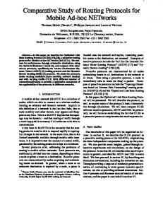
Data packet delivery ratio

TABLE II Fuzzy combination of αc(t) and

Random way point, random walk Constant bit rate 50 m Pause time 10 sec, speed 0-50m/sec 4000m 300m, 2000m 1600m 40, 80, 160, 250, 400 500 sec 5 sec

100 95

Original-DSR

90

QLR-DSR

85

PATCH-DSR

80

LRR-DSR FLRR-DSR

75 70 40

80 160 250 Num ber of nodes

400

Fig 1. Graphical representation of data delivery ratio vs number of nodes

Simulations were carried out using ns-2 [11, 12], a well known packet level simulator, to evaluate the proposed local recovery mechanism. The original DSR in ns is extended to include PATCH, QLR, LRR and FLRR. Performance of original DSR is compared with PATCH-embedded DSR (PATCH-DSR), QLR embedded DSR (QLR-DSR), LRR-embedded DSR (LRR-DSR) and FLRR embedded DSR (FLRR-DSR) in figures 1, 2, 3, 4, 5 and 6. The simulation parameters are presented in table VII.

8

International Journal of Computer Applications (0975 – 8887) Volume 7– No.6, September 2010

30

Control overhead

7000 6000

Original-DSR

5000

QLR-DSR

4000

PATCH-DSR

3000

LRR-DSR

2000

FLRR-DSR

1000 0 80 160 250 Num ber of nodes

400

50000

Consumed energy

Original-DSR

20

QLR-DSR

15

PATCH-DSR

10

LRR-DSR FLRR-DSR

5

40

Fig 2. Graphical representation of control overhead vs number of nodes

40000

Original-DSR

30000

QLR-DSR PATCH-DSR

20000

LRR-DSR

10000

FLRR-DSR

0 40

80 160 250 Num ber of nodes

400

Fig 3. Graphical representation of energy consumption vs number of nodes Average delay in route-repair

25

0 40

2 Original-DSR

1.5

QLR-DSR 1

PATCH-DSR LRR-DSR

0.5

FLRR-DSR

0 40

80 160 250 Num ber of nodes

400

Fig 4. Graphical representation of average delay in route-repair vs number of nodes

Average end-to-end delay

Average hop count

8000

6 5

Original-DSR

4

QLR-DSR

3

PATCH-DSR

2

LRR-DSR FLRR-DSR

1 0 40

80 160 250 Num ber of nodes

400

Fig 5. Graphical representation of average end-to-end delay vs number of nodes

80 160 250 Num ber of nodes

400

Fig 6. Graphical representation of average hop count vs number of nodes

The results are averaged over 30 sets of simulation results and plotted at 95% confidence interval. At low node density in the network, none of the mentioned recovery schemes show much advantage. Especially when the number of nodes is as low as 40, the connectivity of the whole network is not quite good and the problem of partitioning may be severe. Most of the transmission is successful only in small partitions with short route length. In such situation, the local recovery covers most portion of the whole partition already, thus we cannot see obvious control packet saving at low density. However, as the density goes higher, the connectivity of the network becomes higher; transmission with longer route length can be formed at this stage. In such situations, local recovery schemes start to show obvious improvement over end-to-end recovery scheme, as local recovery floods the route repair request in a small region whereas end-toend recovery floods the entire network. Moreover, unlike QLR, PATCH and LRR, FLRR is concerned with stability of links and remaining charge as well as rate of energy depletion of the nodes. Hence, control overhead in FLRR embedded version of DSR is much smaller compared to their ordinary version and QLR, LLR and PATCH embedded versions. Less control overhead yields less energy consumption and less network congestion as well. Decrease in network congestion greatly reduces the possibility of packet collision. As a result, percentage of successful packet delivery ratio increases significantly. For all the above-mentioned protocols, packet delivery ratio is low when the number of nodes in the network is as low as 40. Then it starts increasing till the network is saturated with nodes after which the delivery ratio goes down again. The reason is that, initially the network is partitioned and lots of data packets fail to reach the destination due to unavailability of routes. The situation gradually repairs as the node density increases. After that, when the network gets saturated with nodes, collision among the packets destroy some data packets before they arrive at the destination. As far as delay in route-repair and end-to-end delay are concerned, FLRR produces huge improvement compared to ordinary DSR because ordinary DSR always goes for end-to-end route discovery instead of local recovery as in FLRR, LRR, QLR and PATCH. After a link breakage, all three of LRR, QLR and PATCH communicate through the first available alternative. On the contrary, FLRR waits for a predefined threshold time interval TINV, and chooses the optimal one out of the options available. The optimality criteria consist of remaining energy of nodes, their rate of depletion of energy and stability between 9

International Journal of Computer Applications (0975 – 8887) Volume 7– No.6, September 2010 consecutive links. Preferring the stable links reduce the possibility of further link breakages in that session. Hence the number of occurrences of link breakage in FLRR embedded DSR is much less than LLR, QLR and PATCH embedded versions of DSR. This results in the reduction of delay in route-repair per session and delay in completion of a communication session or end-to-end delay. As far as average hop count is concerned, there is not much difference among the above mentioned protocols. In summary it can be said that, FLRR embedded version of DSR produces much better performance than ordinary DSR, QLRDSR, PATCH-DSR and LRR-DSR while keeping the average hop count very close to one another.

[3] Tsu Wei Chen and Mario Gerla, “Global State Routing: A new Routing Scheme for Ad Hoc Wireless Networks”, Proceedings of IEEE International Conference on Communications, 1998

5. COMPLEXITY ANALYSIS

[7] W. Su and M. Gerla, “IPv6 flow handoff in ad hoc wireless networks using mobility prediction”, Proceedings of IEEE GlobeComm 1997, pp. 271-275

In order to find efficiency of an alternative path option na nc ne, FLRR requires access to each of the tables II to VI exactly once while table I is accessed 7 times (for each of the inputs αc(t), ac(t), ce(t), ac(t), ce(t), ra and rc). Hence, total 12 table accesses are required for each path options. Assuming that the threshold waiting time interval be TINV and one path option can arrive in unit time, efficiency of at most TINV number of paths may have to be computed before selection of the optimal one. So, the overall complexity is (12 TINV).

[4] Hong Jiang, “Simulation of source tree adaptive routing”, March 2000 [5] David B. Johnson, David A. Maltz, “Dynamic source routing in ad hoc networks”, Mobile Computing, pp. 153181 [6] Yu Chen kuo et. Al, “A lightweight routing protocol for mobile target detection in wireless sensor networks”, In proceedings on NCM 2009

[8] Chai Keong Toh, “Associativity – based routing for ad hoc networks”, IEEE International Phoenix Conference on Computers and Communications (IPCCC’96) [9] Joo-Sung Youn, et. Al.,“Quick Local Repair using adaptive promiscuous mode in mobile ad hoc networks”, Jounal of Networks, vol. 1, no. 1, May 2006

6. REFERENCES

[10] Genping Liu et. Al.,”PATCH: A novel local recovery mechanism for mobile ad hoc networks”, IEEE WCNC 2003

[1] Charles E. Perkins, “Highly dynamic destination sequenced distance vector routing for mobile computers”, ACM Computing and Communications Review, vol. 14, issue 4, pp. 234 – 244

[11] Natarajan Meghanathan, “An effective localized route-repair algorithm for use with unicast routing protocols for mobile ad hoc networks”, International Journal of Computer and Network Security, vol. 1, no. 2, November 2009

[2] Shree Murthy, J.J. Garcia-Luna-Aceves, “An efficient routing protocol for wireless networks”, Mobile Networks and Applications (Kluwer Academic Publishers), pp. 183197, 1996

[12] http://www.isi.edu/nsnam/ns

10