20 Oct 2000 - Flockhart and Dhariwal [25] measured the flow characteristics of distilled ...... [1] Frank P. Incropera, David P. Dewitt, Fundamentals of Heat and ...
17 Fluid Dynamics in Microchannels Jyh-tong Teng et al.*
Department of Mechanical Engineering Chung Yuan Christian University, Chung-Li Taiwan 1. Introduction 1.1 Need for microchannels research In contrast to external flow, the internal flow is one for which the fluid is confined by a surface. Hence the boundary layer develops and eventually fills the channel. The internal flow configuration represents a convenient geometry for heating and cooling fluids used in chemical processing, environmental control, and energy conversion technologies [1]. In the last few decades, owing to the rapid developments in micro-electronics and biotechnologies, the applied research in micro-coolers, micro-biochips, micro-reactors, and micro-fuel cells have been expanding at a tremendous pace. Among these micro-fluidic systems, microchannels have been identified to be one of the essential elements to transport fluid within a miniature area. In addition to connecting different chemical chambers, microchannels are also used for reactant delivery, physical particle separation, fluidic control, chemical mixing, and computer chips cooling. Generally speaking, the designs and the process controls of Micro-Electro-MechanicalSystems (MEMS) and micro-fluidic systems involved the impact of geometrical configurations on the temperature, pressure, and velocity distributions of the fluid on the micrometer (10-6 m) scale (Table 1.1). Therefore, in order to fabricate such micro devices effectively, it is extremely important to understand the fundamental mechanisms involved in fluid flow and heat transfer characteristics in microchannels since their behavior affects the transport phenomena for the bulk of MEMS and micro-fluidic applications. Overall, the published studies based on an extensive literature reviews include a variety of fluid types, microchannel cross-section configurations, flow rates, analytical techniques, and channel materials. The issues and related areas associated with the microchannels are summarized in the following table (Table 1.2). Jiann-Cherng Chu1, Chao Liu2, Tingting Xu2, Yih-Fu Lien1, Jin-Hung Cheng1, Suyi Huang2, Shiping Jin2, Thanhtrung Dang3, Chunping Zhang2, Xiangfei Yu2, Ming-Tsang Lee4, and Ralph Greif5 1Department of Mechanical Engineering, Chung Yuan Christian University, Chung-Li, Taiwan 2School of Energy and Power Engineering, Huazhong University of Science and Technology, Wuhan, China 3Department of Heat and Refrigeration Technology, Hochiminh City University of Technical Education, Hochiminh City, Vietnam 4Department of Mechanical Engineering, National Chung Hsing University, Taichung, Taiwan 5Department of Mechanical Engineering, University of California at Berkeley, CA, USA *
404
Fluid Dynamics, Computational Modeling and Applications
Definition
The range of channel dimension
Conventional channels
Dc>3 mm
Minichannels
3 mm ≧ Dc > 200 μm
Microchannels
200 μm ≧ Dc >10 μm
Transitional Microchannels
10 μm ≧ Dc >1 μm
Transitional Nanochannels
1 μm ≧ Dc >0.1 μm
Nanochannels
Dc≦0.1 μm
Table 1.1. Channel classification schemes [2] General research areas
Related studies
1. Cross-sections of microchannels 1. Size effect (Hydraulic diameter) -Triangle, Rectangle, Trapezoid, Circle, Square 2. Aspect ratio and Non-uniform. 3. Entrance effect 2. Materials of microchannels - Silicon, Nickel, Polycarbonate, Polyamide, Fused silica, Stainless steel, Copper, Aluminum, Brass, Glass, Oxidized silicon, SiO2, Polyvinylchloride, Poly-dimethylsiloxane(PDMS), poly-methyl methacrylate (PMMA). 3. Types of flows - N2, H2, Ar, Water, R-134a, Methanol, Isopropanol, Aqueous KCI, Fluorinert fluid FC-84, Vertrel XF, Air, Helium, Silicon oil.
4. Flow rates - Reynolds number, Mach number
1. Surface roughness 2. Contact angle 3. Hydrophilic and hydrophobic property 4. Electrical double layer (EDL) 5. Thermo-physical properties 1. Polarity 2. Rarefaction effect 3. Compressibility 4. Temperature jump 5. Non-slip and Slip 6. Joule heating 1. Critical Reynolds number of the transition to turbulence 2. Viscous heating or Viscous dissipation 3. Mal-distribution
5. Analytical techniques for microchannel 1. Flow pattern and visualization flows 2. Velocity field - Numerical simulation 3. Temperature distribution - Experimental analysis 4. Friction factor 5. Nusselt number 6. Poiseuille number Table 1.2. Summary of research areas and discussed issues related to fluid flow in microchannel [3]
405
Fluid Dynamics in Microchannels
1.2 Research methodology As the field of micro-fluidic systems continues to grow, it is becoming increasingly important to understand the mechanisms and fundamental differences involved in microscale fluid flow. To study the thermal and hydrodynamic characteristics of fluid flow in microchannels, this work used experimental measure and numerical simulation to investigate the behavior of flow and temperature fields in microchannels. In this chapter, each part of the study will be described separately as follows. 1.2.1 Experimental work To carry out the experiments of the flow in microchannels, first and foremost, a fluid flowing and measurement system, together with microchannel structures should be properly designed and built up. In this study, the details of experimental procedure involving the manufacturing of test chip, construction of experimental system, and analysis of experimental uncertainties will be described in the following sections. In this chapter, an experimental flow chart related to the experimental procedure is shown in Fig. 1.1. Experiment equipment turned on
Liquid flow regulated to obtain desired mass flow rate
Leakage checked
Steady state flow rate noted after 20 min
Temperature and Pressure readings noted Different heat transfer condition adjusted
Minutely readings of P, Tw, Tin, and Tout, noted for 2 hours
Steady state readings checked
Experimental data recorded
Experiment completed
Fig. 1.1. Experimental flow chart [3].
Test section changed
406
Fluid Dynamics, Computational Modeling and Applications
1.2.2 Experimental system The experimental system was divided into three parts – the test section, the water driving system, and the dynamic data acquisition section. In addition, DI water (deionized water) was used as the working fluid. The experimentally-measured data were composed of pressure drop through the microchannel, temperatures of DI water and substrate, and the mass flow rate. Each part of the experimental system will be described separately as follows: 1. Test section Since measuring the local pressure and temperature along the flow path was difficult inside the microchannels, two sumps were machined in the PMMA block and were connected by microchannels with holes made by laser processing. A diaphragm type differential pressure transducer with ranges of 0-35 bars was connected to the sumps to measure the corresponding pressure drop across the inlet and outlet of the microchannel. Concerns had been raised that this kind of fitting could cause some dead volume resulting in the detection of false signals. However, to minimize the dead volume that might appear in the flow channel, extreme caution had been taken to ensure that no visible dead volume was observed there. 2. Water-driven system Precision-controlled fluidic HPLC pump or injection pump was used to transport the DI water through the test section, and the flow rate was controlled in a range from 0.1 to 40 ml/min for the DI water flow. A filter (with a screening size of 0.2 μm) was installed midway to remove any possible particulates and contaminants that might be present in water under testing. For the case with heat generation, the stainless steel plate was electrically heated by directly connecting the bottom of test sections to a DC power supply that provided low voltage and high electric current. Once the working fluid was flowing into the test section, measurements of the pressure drop and temperature were done, followed by the weight measurement of the collected fluid using a precision electronic balance with an accuracy of 0.0001 g to obtain the mass flow rate of the system. In the meantime, the temperature of working fluid in the microchannel was measured by calibrated T-type Cu-Ni thermocouples to determine accurately the values of the water density and viscosity. 3. Dynamic data acquisition section This section used an experimental platform with the test section laying horizontally on the platform, above which a digital microscope hooked with video capture card and signal cable to send the digital image to the PC for data-processing, ensuring that the working fluid passed through microchannel and that no left-over bubbles or impurities existed to block the flow channel that could lead to erroneous signals being obtained for the tests. In the meantime, a notebook PC and a network system were used to transmit data at a speed of one per 500 milliseconds. The data acquisition system for recording the electronic signals was implemented to obtain data from the differential pressure transducer and T-type thermocouples; the system was integrated through the instant monitoring software to record and analyze the data received. For each data point being measured, the flow was considered to be at a steady-state condition when the measured pressure drop and temperature remained unchanged for at least 10 minutes. Each case was repeated for at least three times to make sure that the arrangement could always produce reliable and reproducible results.
407
Fluid Dynamics in Microchannels
1.2.3 Numerical simulation Numerical simulations were done by the CFD-ACE+ software [4] which provided an integrated numerical analysis of the continuity, momentum, and energy equations for the fluid flow and heat transfer. After specifying the boundary condition, CFD-ACE+ uses an iterative, segregated solution method where in the equation sets for variables such as pressure, velocity, and temperature are solved sequentially and repeatedly until a converged solution is obtained. In general, iterative equation solvers are preferred for this task because they are more economical in memory requirements than direct solvers. In CFDACE+ program, conjugate gradient solvers and algebraic multi-grid solver are provided to obtain the converged solution. In Chu et al. [3], the latter method was adopted. The basic idea of a multi-grid solution is to use a hierarchy of grids, from fine to coarse, to solve a set of equations, with each grid being particularly effective for removing errors of the wavelength characteristic of the mesh spacing on that grid. In CFD-ACE+, the finite-volume approach is adopted due to its capability of conserving solution quantities. The solution domain is divided into a number of cells known as control volumes. In the finite volume approach of CFD-ACE+, the governing equations are made discrete and finite, and then numerically integrated over each of these computational cells or control volumes. An example of such a control volume is shown in Fig.1.2 [5].
Fig. 1.2. 3D Computational Cell (Control Volume). The geometric center of the control volume, which is denoted by P, is also often referred to as the cell center. CFD-ACE+ employs a co-located cell-centered variable arrangement, i. e., all dependent variables and material properties are stored at the cell center P. In other words, the average value of any quantity within a control volume is given by its value at the cell center. Most of the governing equations can be expressed in the form of a generalized transport equation as shown in Eq. (1-1), which is also known as the generic conservation equation for a quantity Φ [5]. ( ) t ( V ) ( ) S transient
convection
diffusion
source
(1-1)
408
Fluid Dynamics, Computational Modeling and Applications
where S is the source term. The overall solution procedure in flowchart form for the solution algorithm is shown in Fig. 1.3. The number of iterations (NITER) can be defined to dictate how many times a procedure is repeated [6].
Fig. 1.3. Solution Flowchart.
2. Fundamental theory about flow motion 2.1 Pressure drop in single liquid-phase flow 2.1.1 Basic pressure drop correlations For a non-circular cross section of the flow channels, the calculated hydraulic diameter Dh of a rectangular channel is computed by the following equation: Dh = 4Ach/Pw = 2WH/(W+H)
(2-1)
409
Fluid Dynamics in Microchannels
where Ach, Pw, Dh, W and H represent as the areas of microchannel, wetted perimeter, hydraulic diameter, microchannel width and height, respectively. The Reynolds number Re is defined as: Re mumDh / m
(2-2)
where μm and ρm are mean dynamic viscosity and mean density of fluid at an arithmetic mean temperature (Tm = (To+Ti)/2), respectively. It should be noted that the fluid properties are functions of the temperature and values are obtained from correlations for dynamic viscosity (μ) correlations for dynamic viscosity (μ), thermal conductivity (k), specific heat (cp), and density (ρ) of DI water. Under actual conditions, the measured pressure drop includes the effect of the losses (1) in the bends and (2) at the entrance and exit, together with the frictional pressure drop in the microchannel. Phillips [7] suggested that the measured pressure drop was the sum of these components.
Pt =
um2
4f app L 2 Kc +K e +2(Ach /Ap ) K 90 + 2 Dh
(2-3)
where ∆Pt, Ap, Kc, Ke, K90, fapp and L are measured pressure drop, plenum area, contraction loss coefficient, expansion loss coefficient, bends loss coefficient and apparent friction factor, respectively. The loss coefficient K90 was recommended by Phillips [7]. Kc and Ke can be obtained from Kays and London [8]. According to the published investigations with regard to microchannels [9-12], these values of loss coefficient are usually obtained from the traditional relationships in macro-scale flow. In addition, the method described above for determining minor losses was supported by the data obtained by Abdelall et al. [13], which showed that the experimentally measured loss coefficients associated with single-phase flow in abrupt area changes in microchannels were comparable to those obtained for large channels with the same area ratios. 2.1.2 Pressure drop in fully-developed laminar flow For hydrodynamically fully developed flow, the velocity gradient at the channel wall can be readily calculated from the well-known Hagen-Poiseuille parabolic velocity profile for the fully developed laminar flow in a pipe. The Fanning friction factor fc is expressed in the following form:
fc = Po/Re
(2-4)
where the Poiseuille number Po is defined as Po = fRe, the product of the friction factor and the Reynolds number. For incompressible flow through horizontal channels of constant cross-sectional area, fc can be calculated by Eq. (2-5), based on the mass flow rate and the pressure drop ∆P where the latter is due to the friction occurred inside the rectangular microchannel. fc
2 w Dh P mum2 2 mum2 L
(2-5)
where τw is the wall shear stress, L is the channel length, and um is the mean flow velocity.
410
Fluid Dynamics, Computational Modeling and Applications
A simple equation proposed by Shah and London [14] for fully developed, incompressible and laminar flow in a rectangular channel was used to predict the friction factor of straight rectangular microchannels. This equation, which has been used and proven to be adequate for predicting liquid flows in rectangular microchannels by several researchers [15-17], is expressed as follows:
f c 24(1 – 1.3553 c +1.9467 c 2 – 1.7012 c 3 +0.9564 c 4 – 0.2537 c 5 ) / Re
(2-6)
Here fc is the Fanning friction factor for a straight channel and αc is the aspect ratio, which is the ratio of the dimension for the short side to that of the long side. 2.1.3 Pressure drop in developing laminar flow The hydrodynamic entry length Lh for rectangular microchannels is given as follows [2]. Lh / Dh 0.05Re
(2-7)
The apparent friction factor (fapp) includes the combined effects of frictional losses (pressure losses in developed region) and the additional losses in the developing region. The difference between the apparent friction factor (fapp) over a length x, measured from the entry location, and the fully developed Fanning friction factor (fc) is expressed in terms of an incremental pressure defect K(x) as follows [3]: K( x )
f app fc (4x ) / Dh
(2-8)
where K(x) is the Hagenbach factor in the above equation. 2.1.4 Fully developed and developing turbulent flow Regarding fully developed turbulent flow in smooth microchannels, a number of correlations with comparable accuracies are available in the literatures. Blasius put forward the following equation which is used extensively nowadays. f 0.0791Re 0.25
(2-9)
Covering both the developing and developed flow regions, Phillips [18] used a more accurate equation for Fanning friction factor in a circular tube. f ARe B
(2-10)
1.01612 0.32930 and B 0.26800 x / Dh x / Dh For rectangular microchannels, Re is replaced with the laminar-equivalent Reynolds number given by
where A 0.09290
Re *
umDle um[(2 / 3) (11 / 24)(1 / c )(2 1 / c )]Dle
where Dle is the laminar-equivalent diameter calculated by the term in the brackets.
(2-11)
411
Fluid Dynamics in Microchannels
2.1.5 Laminar-to-turbulent transition The laminar-to-turbulent flow transition is another topic investigated by lots of researchers. In the entrance region of rectangular tubes with abrupt area change, the laminar-toturbulent transition was reported to take place at a transition Reynolds number of Ret = 2200 for αc =1 and at Ret = 2500 for parallel plates with αc =0. For the other aspect ratios, a linear interpolation is recommended. Some of the initial studies presented an early transition to turbulent flow in microchannels. However, several recent studies stated that the laminar-to-turbulent transition remained unchanged. For circular microtubes with diameter 171-520 μm, Bucci et al. [19] pointed that the transition occurred around Ret = 2000. The result of Baviere et al. [20] also indicated that the dimensions of smooth microchannels didn’t affect the laminar-to-turbulent transition and the critical Reynolds number was still around 2300. It can be supported by a number of investigators, such as Schmitt and Kandlikar [21] for minichannels with Dh<1 mm, and Li et al. [22] for 80 μm ≤ Dh ≤ 166.3 μm. 2.1.6 Pressure drop related to the change liquid properties Eq. (2-6) provides the theoretical value of Fanning friction factor in rectangular microchannels at constant thermal properties of liquid suggested by Shah and London [23]. In the present experiments, the effect of liquid property variations cannot be neglected for a large temperature difference between inlet and outlet. Kays and London [8] suggested a corrected correlation for temperature dependent properties.
f / fm
w / m M
(2-12)
where M = 0.58 for liquid heating, and M = 0.5 for liquid cooling; subscripts m and w are for the condition at the arithmetic mean fluid temperature and the condition at the wall temperature, respectively. Then, the corrected form for the Shah and London correlation [23] according to the present study is f c ’ f c w / m
M
(2-13)
2.2 Basic heat transfer correlations in single liquid-phase flow Results for the total heat transfer rate and the axial distribution of the mean temperature are derived as follows for the constant surface temperature condition (taking three heated walls in a channel for example, as shown in Fig. 2.1). Defining ∆T as Ts – Tm, the equation may be expressed as dTm d( T ) Pw hT p dx dx mc
(2-14)
Separating variable and integrating from the tube inlet to the outlet yield To
T
i
or,
L P d( T ) w hdx 0 mc p T
(2-15)
412
Fluid Dynamics, Computational Modeling and Applications
ln(
To P L L1 ) w dx p 0 L Ti mc
(2-16)
From the definition of the average convection heat transfer coefficient, it follows that ln(
To P L A ) w hL s hL , p p Ti mc mc
Ts = constant
(2-17)
where hL , or simply h , is the average value of h for the entire channel, As is the heat exchange area between the working fluid and wall surface inside the channel. Rearranging, A To Ts Tm , o exp( s h ) , p mc Ti Ts Tm , i
Ts = constant
(2-18)
For a general form of Eq. (2-18), one can obtain Ts Tm ( x ) P x exp( w h ) , p Ts Tm ,i mc
Ts = constant
(2-19)
Fig. 2.1. Flow through a rectangular microchannel. Since, by definition, Nusselt number equals to h·Dh/λ, the average value of Nu for the entire channel can be expressed as Nu
Dh
m
p T mc ln o , Ti As
Ts = constant
(2-20)
where λm and cp are the mean thermal conductivity and heat capacity at constant pressure of DI water at an arithmetic mean temperature, respectively; As is the heat exchange areas between the walls and fluid.
Fluid Dynamics in Microchannels
413
For the heat exchange at the constant heat flux, the deduction of correlations can be found in [1]. Moreover, Lee et al. [24] examined the validity of conventional correlations and numerical analysis approaches in predicting the heat transfer behavior in microchannels for correctly matched inlet and boundary conditions.
3. Flow and heat transfer in microchannels of various configurations 3.1 Flow and heat transfer in V-shaped microchannels A number of experimental and numerical investigations of single phase flow in microchannel have been extensively performed. However, most studies have experimental results obtained for microchannels with rectangular and circular crosssections. The studies of thermo-fluidic characteristics in microchannels with a V-shaped cross-section are quite limited in this field. Thus, it is necessary to provide the present knowledge of V-shaped microchannel. Flockhart and Dhariwal [25] measured the flow characteristics of distilled water inside trapezoidal microchannels with hydraulic diameters ranging from 50 to 120 μm and the Reynolds numbers below 600. They found that the flow characteristics of water in trapezoidal microchannels could be predicted by the numerical analysis based on the conventional theory. Qu et al. [26, 27] used experimental and theoretical methods for the study of the thermofluidic characteristics of the trapezoidal microchannels with hydraulic diameters ranging from 62 to 169 m. Results of their study indicated that the wall roughness of the microchannels might lead to lower Nusselt numbers as comparing with those obtained from the theoretical predictions. In addition, they also found that the experimentally determined friction factors in the trapezoidal microchannels were higher than those obtained from the conventional theory. They used a roughness-viscosity model developed by Mala and Li [16] to interpret the difference of friction factors obtained from the experimental data and those obtained from the conventional theory. Hetsroni et al. [28] performed an experimental investigation of a microchannel heat sink for cooling of electronic devices. The heat sink had parallel triangular microchannels with a base of 250 m. The results indicated that the temperature distribution at the exit of the triangular microchannel had a nonlinear distribution, and the instabilities caused fluctuations in the pressure drop and decrease in the heat transfer coefficient. Wu and Cheng [29] conducted a series of experiments to measure the friction factor and convective heat transfer coefficient in trapezoidal silicon microchannels with different surface conditions. The results indicated that the geometric parameters had significant effect on the Nusselt number and Poiseuille number of trapezoidal microchannels, and the hydrophilic property at the surface of the microchannel enhanced the heat transfer capability of the trapezoidal silicon microchannels. Wu and Cheng [30] experimentally studied the laminar flow of de-ionized water in smooth silicon microchannels of trapezoidal cross-sections with hydraulic diameters ranging from 25.9 to 291 m. The measured results indicated that the Navier-Stokes equations were still valid for the laminar flow in the trapezoidal microchannel having a hydraulic diameter as small as 25.9 m. Tiselj et al. [31] performed the experimental and numerical analyses to evaluate the effect of axial heat flux on heat transfer in triangular microchannels with hydraulic diameter of 160 μm in the range of Reynolds numbers from 3.2 to 64. The experimental results revealed that
414
Fluid Dynamics, Computational Modeling and Applications
the temperature distribution of the triangular microchannels on the heated wall was in agreement with the numerical predictions obtained from conventional Navier-Stokes and energy equations. Tiselj et al. [32] used three-dimensional numerical simulations for the study of the heat transfer characteristics of the fluid flowing through triangular microchannels. Their results indicated that a singular point existed near the exit of the channel. In addition, for the flow with higher Reynolds number, the singular point was closer to the exit of the channel. Based on the conventional theory, Morin [33] developed a model to predict the viscous dissipation effects in a microchannel with an axially unchanging cross section. The microchannel geometries having rectangular, trapezoidal, and double trapezoidal were discussed in his work. The water and isopropanol were used as working fluids. The analytical results demonstrated that for different fluids the effect of viscous dissipation could play different roles and that the effect of viscous dissipation could become very significant for liquid flows when the hydraulic diameter was less than 100 μm. In addition, the rising temperature in an adiabatic microchannel could be expressed as a function of the Eckert number (defined as Ec = u2/cvT), Reynolds number, and Poiseuille number. 3.1.1 Model description For the manufacture of V-shaped microchannels, photolithographic processes are particularly utilized for silicon wafers, and these processes initiated in the electronic field are well developed. When a photolithography-based process is employed, the microchannels having a cross-section fixed by the orientation of the silicon crystal planes can be fabricated; for example, the microchannels etched in or in silicon by using a potassium hydroxide (KOH) solution can form a V-shaped cross-section (as shown in Fig.3.1).
(a)
(b)
Fig. 3.1. (a) Flowchart of micro-manufacture processing; (b) V-shaped microchannels.
415
Fluid Dynamics in Microchannels
3.1.2 Results and discussion For incompressible, fully-developed laminar flow, the friction factor can be expressed in terms of the two experimentally obtained parameters – pressure drop and mass flow rate.
fexp
Dh 2 Pexp ( KL ) L Vav 2
(3-1)
where KL is the friction factor for the minor loss. For the comparison of values of f vs. Re as shown in Fig. 3.2, the differences between the results obtained from numerical simulation and those from traditional correlation are within 2.5% of each other, within 6% between the numerical simulations and the experimental data, and with the f vs. Re values obtained from the experimental data and those obtained from the numerical simulations approaching a fixed value which is slightly lower than the value of 53.3 predicted by the traditional theory.
Fig. 3.2. Comparison of f vs. Re for theoretical values, predicted values, and experimental data for Specimen Set No. 4 [3]. Wu and Cheng [29] proposed a correlation for the V-shaped microchannels (Wb/Wt = 0) for fluid at low Reynolds numbers as follows. Nu 6.7 Re
0.946
Pr
0.488
Wb 1 Wt
3.547
Wt H
3.577
Dh
0.041
Dh L
1.369
, Re < 100
(3-2)
416
Fluid Dynamics, Computational Modeling and Applications
where Wb and Wt are the bottom and the top width of microchannel, respectively. And ε is the surface roughness. Referring Wu and Cheng [29], Chu [3] proposed an empirical correlation, based on experimentally obtained data from four sets of triangular microchannel test specimens (with different channel widths) under low Reynolds number conditions (Re < 50). Nu
1 1.2 (-23.1 25.4Wt0.5 )2 Re -2
(3-3)
Generally speaking, the trends of the predicted results obtained from the correlation specified by Eq. (3-3) are in agreement, as shown in Fig. 3.3, while the widths of the microchannels have an obvious impact on the behavior of the development of the Nusselt numbers for the microchannels under study. It is noted that the magnitude of the Nusselt number increases at a slower rate as the Reynolds number becomes larger than 20.
Fig. 3.3. Comparison of Nu vs. Re among empirical correlation and experimental data. It is also noted that high temperature gradients at the inlet and exit were observed from the temperature distributions of microchannels for all sets of the test specimens. In addition, the Nusselt numbers increase as the Reynolds number increases, as shown in Fig. 3.3. For the range of the Reynolds number being tested (Re < 50), the average discrepancy of the values calculated from the correlation of Nu obtained in [3] and those obtained from the experimental data is within 15%; the difference is judged to be in fair agreement.
Fluid Dynamics in Microchannels
417
3.2 Flow in circular curved microchannels Among various micro-fluidic systems such as micro-coolers, micro-biochips, micro-reactors, and micro-fuel cells [3], the curved or bended microchannel (as shown in Fig. 3.5) has been identified as being one of the essential elements for shifting the direction of fluid flow, increasing the length of the path of the fluid flow, enhancing mixing efficiency, and improving heat transfer performance within a confined and compact space [24-26]. Therefore, it is extremely important to acquire a fundamental understanding of the flow behavior of fluid in curved microchannels, since its behavior affects the transport phenomena for the design and process control of micro-fluidic systems. Up to the present time, there have been numerous investigations in the characteristics of the flow inside straight microchannels. However, a review of the literatures relative to researches conducted in straight microchannels during the last decade [37, 38] has revealed that only a handful of experimental or computational evaluations were done on the study of flow characteristics in curved microchannels [39-41]. For the manufacture of curved microchannels, Chu [3] demonstrated that the curved microchannel could be constructed by standard etching processes; the curved microchannel was etched on a silicon wafer with a 4-inch diameter and a 550 m thickness. The processes included SiO2 deposition, photoresist coating, developing, baking, etc. Subsequently, an inductively coupled plasma (ICP) process accounting for the crystal directional characteristics was used to finish the fabrication of the curved microchannel structure (as shown in Figs. 3.4 and 3.5).
Fig. 3.4. Process flow of fabrication for curved rectangular microchannels.
418
Fluid Dynamics, Computational Modeling and Applications
Fig. 3.5. Schematic diagram of the geometry for the curved rectangular microchannel. For curved microchannels, the geometrical configurations used for testing are given in Table 3.1 [3]. Channel type C1 C2 C3 C4 C5 C6 C7 C8 C9 C10 C11 C12 C13 C14 C15
Channel width, w (μm) 200 200 300 300 300 400 400 400 200 200 200 300 300 400 400
Channel height, h (μm) 200 200 200 200 200 200 200 200 40 40 40 40 40 40 40
Radius of curvature, Rc (μm ) 5,000 10,000 5,000 7,500 10,000 5,000 7,500 10,000 5,000 7,500 10,000 7,500 10,000 5,000 10,000
Aspect ratio, αc 1 1 0.667 0.667 0.667 0.5 0.5 0.5 0.2 0.2 0.2 0.133 0.133 0.1 0.1
Curvature ratio 0.04 0.02 0.048 0.032 0.024 0.0533 0.0355 0.0266 0.0133 0.0088 0.0066 0.0094 0.007 0.0146 0.0072
Table 3.1. Geometrical parameters of the curved microchannels used for testing For incompressible flow through horizontal channels of constant cross-sectional area, the Fanning friction factor fc is based on the mass flow rate and the pressure drop ΔPf, where the latter is due to the friction occurred inside the curved microchannel.
419
Fluid Dynamics in Microchannels
fc
2 w D P 180 w 3 h 3 Pf h2 f 2 um 2 umL Rc c Q 2 ( h w)
(3-4)
where w is the wall shear stress, L is the channel length, um is the mean flow velocity, Q is the volumetric flow rate of the working fluid, Rc is the radius of curvature, and θc is the angle of the microchannel. According to the recommendations and method described by Holman [42], Chu [3] proposed the expression of uncertainties associated with Re, f and the product fRe for curved microchannels. 2 2 2 2 U Re Q h w Re Q h w
1/2
2 2 2 2 2 2 2 Q L U f p h w h w 4 9 9 f p h w hw Q L
(3-5)
1/2
2 2 2 2 2 2 2 U f Re p Q L h w h w 9 9 4 fRe p Q L h w hw
(3-6)
1/2
(3-7)
In Eqs. (3-5) – (3-7), it is observed that the measurement errors in the height h and width w of the microchannel dimensions have a significant influence on the overall uncertainty. In order to compare the flow characteristics of the curved microchannel with those of the conventional dimensions, the relationship between the friction factor and the Reynolds number estimated from the empirical correlation proposed by Yang et al. [43] are plotted in Figs. 3.6 and 3.7 (it should be noted that the correlation was originally proposed by Hua and Yang [44]). The correlation is expressed by the following equation. f
5 w Re 0.65 2R c
0.175
(3-8)
From Figs. 3.6 and 3.7, it is observed that when Re