Sep 15, 2009 - Discretize the domain using finite differences. ⢠Define scalar & vector fields on the grid .... Ch
Fluid Simulation Overview Presentation Date: Sep 15th, 2009 Chrissie C. Cui
Outline • • • • • • •
Introduction Fluid Characteristics Navier-Stokes Equation Eulerain vs. Lagragian approach Fluid Simulation Stages Solid Fluid Coupling Read-time fluids
Introduction • Application – – – –
Computer Games Scientific Computation Special Movie Effects Medical Simulation (Blood Flow)
• What can we achieved so far? – – – – –
Smoke Granular flow (sand) Newtonian fluid (Water, ocean) Non-Newtonian fluid (Blood, Honey) Microscopic phenomena
Characteristics - Basic Fluid Properties • Vector Field – Velocity (v) – Pressure (p) – Additional Force (f) – Surface Tension (t)
• Scalar Field – Density (ρ) – Viscosity (ѵ)
Characteristics – Fluid Types • Incompressible vs. Compressible Fluids – Incompressible Fluids: Fluids doesn’t change volume very much – Compressible Fluids: Fluids change their volume significantly
• Viscous vs. Inviscid Fluids(ideal): – Viscous Fluids: Fluids tend to resist a certain degree of deformation – Inviscid Fluids: Fluids don’t have resistance to the shear stress
• Turbulent vs. Laminar (streamline) Flow: – Turbulent Flow: Flow that appears to have chaotic and random changes – Laminar Flow: Flow that has smooth behavior
• Newtonian vs. Non-Newtonian Fluids: – Fluids continue to flow, regardless of the force acting on it – Fluids that have non-constant viscosity
Naiver-Stokes Equation • Momentum Equation
ut = k∇2u –(u⋅∇)u – ∇p + f Change in Diffusion/Vi Advection velocity scosity
• Incompressibility
∇⋅u=0
Pressure
Body Forces
u: the velocity field k: kinematic viscosity
• Common techniques for solving Navier Stoke’s equation: – – – –
Eulerian approach (grid-based) Lagrangian approach (particle-based) Spectral method Lattice Boltzmann method
Eulerian Approach • Discretize the domain using finite differences • Define scalar & vector fields on the grid • Use the operator splitting technique to solve each term separately • Evaluation: Derivative approximation Adaptive time step/solver Memory usage & speed Grid artifact/resolution limitation
Lagrangian Approach • Treat the fluid as discrete particles • Apply interaction forces (i.e. pressure/viscosity) according to certain pre-defined smoothing kernels • Evaluations: Mass / Momentum conservation More intuitive Fast, no linear system solving Connectivity information/Surface reconstruction
Fluid Simulation Stages – Main Loop
Fluid Simulation Stages – Advection I • • • •
Sometimes called “Convection” or “Transport” Define how a quantity moves with the underlying velocity field This term ensures the conservation of momentum Advection equation:
ut = −(u ⋅ ∇u ) • Approaches: – Forward Euler (unstable) – Semi-Lagragian advection (stable for large time steps, but suffers from the dissipation issue)
Fluid Simulation Stages – Advection II
Fluid Simulation Stages – Diffusion I • Define how a quantity in a cell inter-changes with its neighbors • Diffusion = Blurring • The viscous fluid can be achieved by applying diffusion to the velocity field Low Viscosity
High Viscosity
Figures from [Carlson, Mucha, Turk] Melting and Flowing, SCA 02
Fluid Simulation Stages – Diffusion II 1
• Diffusion equation:
ut = k ⋅ ∇ u 2
1
• Approaches:
-4
1
1
– Explicit formulation ut = k ⋅ ∆t ⋅ (ui +1, j + ui −1, j + ui , j +1 + ui , j −1 − 4 ⋅ ui , j )
– Implicit formulation (for high viscosity) u n i , j = u n +1i , j − k ⋅ ∆t ⋅ (u n +1i +1, j + u n +1i −1, j + u n +1i , j +1 + u n +1i , j −1 − 4 ⋅ u n +1i , j ) Unknowns
Fluid Simulation Stages – Diffusion III
Fluid Simulation Stages – Pressure Solver I • It’s sometimes called “Pressure Projection” • What does the pressure do? – Keep the fluid at constant volume (incompressible, conservation of mass). – Make sure the velocity field stays divergence-free
∑ flux = 0 all _ faces
Incompressible
Compressible
Fluid Simulation Stages – Pressure Solver II • Equation to solve: u
n +1
=u − n
1
ρ
∇p
s.t.
∇ ⋅u
n +1
=0
• • • (1)
Unknowns
• How to solve for pressure: – Taking divergence of both sides of (1), we will have
1
ρ
∇2 p = ∇⋅ un
(Poisson Equation)
– Build a system of equations and solve Ap = d using an iterative method such as Conjugate Gradient – Update the velocity field from the pressure gradient
Fluid Simulation Stages – Pressure Solver III • What about the pressure on boundary nodes? – Free surface: The fluid can evolve freely (p = 0) – Solid wall: The fluid can’t penetrate the wall but can flow freely in tangential directions (Neumann BC)
uboundary ⋅ n = usolid ⋅ n
Solid Fluid Coupling • One-way coupling: – Solid-Fluid interaction: The fluid has no influence on the solid – Fluid-Solid interaction: The solid has no influence on the fluid
• Two-way coupling: – Manipulate the boundary conditions – Finite Element techniques: ALE & DLM – Rigid Fluid: Treat the solid as fluids and enforce the rigidity constraint
• Principles: – – – – –
Real-time Fluids H(x,y)
Cheap to compute Low memory consumption Stability Plausibility Interactivity
• Common techniques: – Procedural water: Superimpose sine waves of a variety of amplitudes and directions. – Height field approximations: If the surface is the only interest, it can be represented using a 2D height field and animated by 2d wave equations with interaction forces – Particle systems: This approach is good at simulating a small amount of water such as a puddle, a bubble or splashing fluids k k 1 2 ⋅ xi − x j f (x i , x j ) = − x − x m x − x n xi − x j j i j i
Agenda • Sep 15th - Particle-Based Fluid Simulation for Interactive Applications
• Sep 15th - Hardware-Aware Analysis and Optimization of Stable Fluids
• Sep 22nd – Direct Forcing for Lagrangian Rigid-Fluid Coupling
• Sep 22nd – Directable, High-Resolution Simulation of Fire on the GPU