Formal Foundations of 3D Geometry to Model Robot Manipulators - Inria

Formal Foundations of 3D Geometry to Model Robot Manipulators Reynald Affeldt, Cyril Cohen

To cite this version: Reynald Affeldt, Cyril Cohen. Formal Foundations of 3D Geometry to Model Robot Manipulators. Conference on Certified Programs and Proofs 2017, Jan 2017, Paris, France.

HAL Id: hal-01414753 https://hal.inria.fr/hal-01414753 Submitted on 12 Dec 2016

HAL is a multi-disciplinary open access archive for the deposit and dissemination of scientific research documents, whether they are published or not. The documents may come from teaching and research institutions in France or abroad, or from public or private research centers.

L’archive ouverte pluridisciplinaire HAL, est destin´ee au d´epˆot et `a la diffusion de documents scientifiques de niveau recherche, publi´es ou non, ´emanant des ´etablissements d’enseignement et de recherche fran¸cais ou ´etrangers, des laboratoires publics ou priv´es.

Formal Foundations of 3D Geometry to Model Robot Manipulators Reynald Affeldt

Cyril Cohen

Information Technology Research Institute, National Institute of Advanced Industrial Science and Technology, Japan

MARELLE project-team, INRIA Sophia Antipolis, France

Abstract

1.

We are interested in the formal specification of safety properties of robot manipulators down to the mathematical physics. To this end, we have been developing a formalization of the mathematics of rigid body transformations in the C OQ proofassistant. It can be used to address the forward kinematics problem, i.e., the computation of the position and orientation of the end-effector of a robot manipulator in terms of the link and joint parameters. Our formalization starts by extending the Mathematical Components library with a new theory for angles and by developing three-dimensional geometry. We use these theories to formalize the foundations of robotics. First, we formalize a comprehensive theory of three-dimensional rotations, including exponentials of skewsymmetric matrices and quaternions. Then, we provide a formalization of the various representations of rigid body transformations: isometries, homogeneous representation, the Denavit-Hartenberg convention, and screw motions. These ingredients make it possible to formalize robot manipulators: we illustrate this aspect by an application to the SCARA robot manipulator.

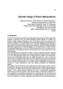
Our ultimate goal is the formal verification of safety properties of robots. Robots have already made their way in manufacturing plants into the form of robot manipulators on assembly lines. Even though industrial robots operate in a controlled environment, their safety is already subject to several standards (e.g., ISO 10218). Safety concerns will increase furthermore now that robots are considered for life-critical missions such as rescue and health care. It is therefore questionable whether testing can achieve a satisfactory level of safety. For this reason, formal methods are now being considered to improve the rigor of the safety analysis of robots (see Sect. 11 for examples). In this paper, we focus on the formal verification of the theoretical foundations of robot manipulators. Robot manipulators are an interesting target because they are already pervasive in the industry and because advanced robots such as humanoid robots can be understood as made of several robot manipulators. The theoretical foundations of robot manipulators is a matter of three-dimensional geometry. This suggests the use of a proof-assistant to perform formal verification. Indeed, proof-assistants excel at the symbolic manipulation of formal algebra, in which geometry can be represented. We use the C OQ proof-assistant (The Coq Development Team 1999–2016) and the Mathematical Components library. The latter is a library for formal algebra that was developed to formalize the odd order theorem, an important theorem in group theory (Gonthier et al. 2013). This library features in particular a formalization of linear algebra that we use as a starting point. We discuss in Sect. 12 the consequences of this choice. Let us give a concrete idea of the kind of three-dimensional geometry robotics is dealing with. A robot manipulator consists of (rigid) links connected by joints. It is modeled by the relative positioning of frames attached to its links. Figure 1 is a schematic representation of the SCARA robot manipulator for pick-and-place operations. It consists of fives links (from the base link 0 to the end-effector—link 4) connected by four joints. The first two joints and the last one

Categories and Subject Descriptors F.4.1 [Mathematical Logic]: Mechanical theorem proving; I.1.1 [Expressions and Their Representation]: Representations (general and polynomial); I.2.9 [Robotics]: Manipulators; I.3.5 [Computational Geometry and Object Modeling]: Hierarchy and geometric transformations Keywords Formal verification, Proof-assistant, Coq, Robot manipulator, 3D Geometry

Towards a Formal Theory of Robotics

a2 a1

link 2

link 1

θ1

θ2 link 3 link 0

θ4

d3 d4 link 4

Figure 1: SCARA robot manipulator (with link and joint parameters)

are revolute joints: they can rotate around one axis (here, the vertical axis). The third joint is a prismatic joint: it can translate along one axis (here, the vertical axis). The rotation angles and the translation distance are called the joint parameters. Reasoning about a robot manipulator amounts to determining the relative positions of links. To do so, one attaches frames to links, often near a joint, as illustrated in Fig. 2. The orientation of a frame z0 z w.r.t. another is expressed y0 1 y1 z2 y2 by a rotation. For exx2 x0 x1 ample, the orientation of z3 y3 frame 1 w.r.t. frame 0 can be expressed by the z4 y4x3 0 R = following matrix h cos θ1 sin θ1 0 i 1 x4 − sin θ1 cos θ1 0 , where 0 0 1 Figure 2: SCARA robot θ1 is the angle of the romanipulator (with the frames tation of the first joint. The hxi , yi , zi i) relative position of a frame w.r.t. another is expressed by a rigid body transformation. For example, the coordinate of the origin of the frame 1 w.r.t. frame 0 is 1 P 0 = [a1 cos θ1 ; a1 sin θh1 ; 0]. The i relative position of frame 1 w.r.t. 0 0 1R 0 frame 0 is 1 A = P 0 1 (row-vector convention)1 . 1 Once the relative positions of links are determined, we can address the forward kinematics problem, i.e., determining the position and orientation of the end-effector of a robot manipulator given the link and joint parameters. For our example, given the relative positions i+1 Ai of the consecutive frames, the position and orientation of the end-effector are given by the matrix product 4 A3 3 A2 2 A1 1 A0 . We further develop this example in Sections 8.3, 9.2, and 10.3. The main contribution of this paper is to provide a formalization of the theoretical foundations of robot manipulators rich enough to address the forward kinematics problem. This requires to formalize a large amount of three-dimensional geometry because robotics uses a wide variety of representations for rotations and rigid body transformations related by 1 It

is customary to represent three-dimensional vectors and rotations by vectors of size 4 and 4 × 4-matrices referred to as their homogeneous coordinates (see Sect. 8).

non-trivial mathematical properties. We can summarize our technical contributions as follows: • We propose a formalization of angles and trigonometric functions based on complex numbers (Sect. 2). This algebraic approach helps us to manage the complexity of the formalization of three-dimensional geometry. • We extend the Mathematical Components library with support for the dot-product and formalizations of the crossproduct, lines, orthogonal (and rotation) matrices, and frames (Sect. 3). • We provide a formal definition of rotations and show equivalence with rotation matrices (Sect. 4), exponential coordinates (Sect. 5), and other representations such as quaternions (Sect. 6). • We formalize various representations of rigid body transformations: as isometries (Sect. 7), as elements of the special Euclidean group using their homogeneous representation (Sect. 8), using the Denavit-Hartenberg convention more specific to robotics (Sect. 9), and as screw motions (Sect. 10). • We address the forward kinematics problem for the SCARA robot manipulator to illustrate the above libraries (Sections 8.3, 9.2, and 10.3). This paper is organized as the progressive presentation of our technical contributions illustrated with the running example of the SCARA robot manipulator. We also comment on related work in Sect. 11 and conclude and discuss improvements and applications in Sect. 12. We assume some familiarity with the C OQ proof-assistant. We display formal definitions verbatim, using only a few standard non-ASCII characters to ease reading. We explain notations when they are introduced. Let us recall some notations of the Mathematical Components library for convenience: a *: v x *+ n x ˆ+ n `|x| x \in A, x \is A n%:R x == y

2.

v scaled by a n times x x to the nth power norm of x x satisfies the predicate A notation for 1 *+ n boolean equality between x and y

Angles and Trigonometric Functions

We start with an overview of a formalization of angles and trigonometric functions that we have been developing in particular to define formally rotations (in Sect. 4). Due to technical reasons explained in Sect. 12, we formalize angles and trigonometric functions on top of real closed fields from the Mathematical Components library (Cohen 2012b). 2.1

Formalization of Angles using Complex Numbers

Angles are defined using algebraic complex numbers of unit norm. In Mathematical Components, the type of complex numbers is R[i], where R is a real closed field (rcfType). An angle is defined as a complex number with norm 1:

function arcsin(x) arccos(x) arctan(x)

formalization in C OQ

pencil-and-paper definition √ arg( 1 −√x2 + xi) arg(x + i 1 − x2 ) arg(sgn(x)( x1 + i)) (0 if x = 0) Table 1: Formalization of inverse trigonometric functions

arg (Num.sqrt (1 - x^2) +i* x) arg (x +i* Num.sqrt (1 - x^2)) if x == 0 then 0 else arg ((x^- 1 +i* 1) *~ sgz (x))

Variable R : rcfType. Record angle := Angle { expi : R[i]; _ : `| expi | == 1 }.

In particular, the argument of a complex number defines an angle: Definition arg (x : R[i]) : angle := insubd angle0 (x / `| x |).

(angle0 is the 0 angle corresponding to the complex number 1; insubd is a Mathematical Components operator that tries to coerce to a sub-type and returns the given default value if it fails; division by 0 in Mathematical Components outputs 0 by convention.) We show that angles form an additive group (so that we can scale angles to obtain, e.g., double-angles in Sect. 6.2, lemma quat_rot_isRot) and we define half-angles (used, e.g., in Sect. 10.2, lemma etwist_is_onto_SE). Specific angles are defined as the arguments of specific complex numbers. For example, we define π as the argument of −1: Definition pi := arg (- 1).

2.2

Trigonometric Functions and Trigonometric Laws

The foundations of robot manipulators make use of a number of trigonometric functions. For example, arccos is used in Sect. 6.1 to define the angle-axis representation, arctan in Sect. 6.2 to define rotations using quaternions, and cotangent in Sect. 10.2 to prove the surjectivity of the exponential of a twist. Technically, we define the functions cos and sin using the real and imaginary parts of the complex numbers that define angles, the functions tan and cot follow: function cos(a) sin(a) tan(a) cot(a)

3.

Basics of Three-dimensional Geometry

3.1

Extended Support to Reason with Vectors

Vectors are provided by the Mathematical Components library in the form of a type denoted by 'rV[R]_n whose elements are row-vectors of length n with components of type R. We distinguish a few specific vectors to simplify notations. In particular, we denote by 'e_0, 'e_1, and 'e_2 the vectors of the canonical basis. Concretely, 'e_k is formalized by the row-vector [δ0k ; δ1k ; δ2k ], where δ is Kronecker symbol. Also, to construct a row-vector from its components, we resort to the row3 constructor ([a; b; c] is represented formally by row3 a b c). 3.1.1

We denote by u ∗d v the dot-product of the vectors u and v. It is formally defined by the only component of the 1 × 1matrix u ∗m v^T, where ∗m is matrix multiplication and ^T is matrix transpose. The dot-product is used to define a number of geometrical constructs. Let us introduce the formalization of a few of them that we will use in the forthcoming sections. The norm of a vector u is defined using the square root of the dot-product hu · ui: Definition norm u := Num.sqrt (u ∗d u).

A vector is normalized by scaling it to be of unit norm: Definition normalize v := (norm v)^- 1 *: v.

The normal component of a vector is defined using the dot-product (see Fig. 3): Definition normalcomp v u := v - normalize u ∗d v *: normalize u.

v

formalization in C OQ

v−

Re (expi a) Im (expi a) sin a / cos a (tan a)^- 1

Inverse trigonometric functions are formalized using their definition in terms of complex numbers (see Table 1). To be useful, our formalization of trigonometric functions needs to be equipped with many trigonometric laws. We formalized in particular the cancellation laws between each trigonometric function and its inverse, and many trigonometric identities (Pythagorean identity, double-angle and halfangle formulas, law of cosines and of sines, etc.).

The Dot-Product

1 h ||u|| u

·

1 vi ||u|| u

u

1 h ||u|| u · vi

Figure 3: The normal component of v w.r.t. u 3.1.2

The Cross-Product

The cross-product of two vectors u and v can be defined using determinants: 1 u × v = u0

0 0 u1 u2 v0 v1 v2

0 'e_0 + uv 0

1 0 u1 u2 0 v1 v2

0 'e_1 + uv 0

0 1 u1 u2 0 v1 v2

'e_2

3.3 We use the determinant \det of the Mathematical Components library to formalize the above formula: Definition crossmul u v := \row_(k < 3) \det (col_mx3 'e_k u v). 'e_k are the vectors of the canonical basis introduced in Sect. 3.1. col_mx3 is the concatenation of three row-vectors into a 3 × 3-matrix. We denote crossmul u v by u ∗v v.

The cross-product is useful to define a number of geometrical constructs, such as colinearity: Definition colinear u v := u ∗v v == 0.

The cross-product is also used to build frames (see Sect. 3.4). The pervasive usage of the cross-product in robotics naturally calls for a rich library. We formalized the expected standard lemmas. For illustration, the double cross-product is a technical but useful lemma about the cross-product and the dot-product (used for example in the proof of rodriguesP in Sect. 5.1 and to deal with quaternions in Sect. 6.2): Lemma double_crossmul u v w : u ∗v (v ∗v w) = (u ∗d w) *: v - (u ∗d v) *: w.

3.2

Formalization of Lines

Lines are important to model robot manipulators: they are used for the relative positioning of frames (Sect. 9.1) or for screw axes (Sect. 10). We formally define lines in a parametric way by a pair of a point (belonging to the line) and a vector (the direction of the line): (* Module Line *) Record t := mk { point : 'rV[R]_3 ; vector :> 'rV[R]_3 }.

Given a line l, we denote by \pt( l ) (resp. \vec( l )) the point Line.point l (resp. the vector Line.vector l). We equip lines with several predicates to discuss their properties. The membership predicate is defined so as to use the generic membership predicate \in of the Mathematical Components library. A point p belongs to the line l when the vectors p - \pt( l ) and \vec( l ) are colinear. We introduce this membership definition as a coercion so as to be able to write expressions such as p \in (l : pred _). We also make use of the following relations: two lines are parallel when their vectors are colinear, perpendicular when the dot-product of their vectors is 0, or skew when they are not coplanar. Two lines intersects when they are neither skew nor parallel. In the latter case, there is a constructive proof to find out the intersection point: Definition is_interpoint p l1 l2 := (p \in (l1 : pred _)) && (p \in (l2 : pred _)). Lemma intersects_interpoint l1 l2 : intersects l1 l2 → {p | is_interpoint p l1 l2}.

Orthogonal and Rotation Matrices

A matrix M such that M M T = 1 is orthogonal. An orthogonal 3 × 3-matrix is a rotation matrix when det(M ) = 1. Let us denote by 'O[R]_n the set of orthogonal matrices and by 'SO[R]_3 the set of rotation matrices (formal definition omitted here).   1 0 0 0 cos(a) sin(a) For example, Rx (a) = is a rotation 0 − sin(a) cos(s)

matrix. It is meant to represent a rotation of angle a around the canonical vector [1; 0; 0] (see Sect. 4). It is formally defined as follows (Ry (a) and Rz (a) are defined similarly): Definition Rx a := col_mx3 'e_0 (row3 0 (cos a) (sin a)) (row3 0 (- sin a) (cos a)).

3.4

Formalization of Frames

As highlighted in the introduction, frames are important to model robot manipulators. We define a non-oriented frame with an orthogonal matrix (Sect. 3.3): (* Module NOFrame *) Record t := mk { M :> 'M[R]_3 ; MO : M \is 'O[R]_3 }.

Let f be a non-oriented frame. We denote by i (resp. j, k) the first (resp. second, third) row of the matrix (M f). The vectors i, j, and k are pairwise orthogonal unit vectors and we regard them as forming the frame f. The sign of a nonoriented frame f is defined by \det (M f) (which is equivalent to i ∗d (j ∗v k)) and can only be 1 or −1. When it is 1, the frame is positive (or right-handed): (* Module Frame *) Record t := mk { noframe_of :> NOFrame.t R ; MSO : NOFrame.M noframe_of \is 'SO[R]_3}.

In particular, we denote by can_frame R the (positive) frame consisting of the canonical vectors 'e_0, 'e_1, and 'e_2. We may add an origin to positive frames: (* Module TFrame *) Record t := mk { o : 'rV[R]_3 ; frame_of :> Frame.t R }.

A frame with an origin defines three line-axes. The x-axis of a frame is defined as follows (and similarly for other axes): Definition xaxis R (f : TFrame.t R) := Line.mk (TFrame.o f) (NOFrame.i f).

Frame Built from a Non-Zero Vector We will need to build positive frames given one non-zero vector (for example to define rotations in Sect. 4.1). For this purpose, we provide a module Base that features two functions j and k such that, given a unit vector i, the vectors i, j i, and k i form a positive frame. Concretely, the function j is defined as follows: (* Module Base *) Definition j i := if colinear i 'e_0 then 'e_1 else normalize (normalcomp 'e_0 i).

If i is colinear with 'e_0 then the desired frame can be built using the vectors of the canonical basis. Otherwise, we compute the normal component of 'e_0 w.r.t. i and we normalize to a unit vector. As for the function k i, it is simply defined by the cross-product of i and j i: this guarantees that the frame is positive.

built using the vectors of the frame hnormalize u, j u, k ui (see Sect. 3.4) expressed in the canonical basis.  Conversely, given a rotation matrix, one can always find a vector-axis and an angle such that the corresponding linear application is a rotation. The vector-axis in question is provided by Euler’s theorem:

Rotation Between Frames A rotation matrix can be regarded as a transformation from one frame to another. For example, multiplication by the matrix Rx (a) (Sect. 3.3) transforms a vector whose coordinates are expressed in the frame h[1; 0; 0], [0; cos(a); sin(a)], [0; − sin(a); cos(a)]i to the same vector but with coordinates expressed in the canonical frame. More generally, let us denote by A _R^ B the rotation matrix that transforms a vector expressed in frame A into a vector expressed in frame B; it is defined as follows:

Lemma euler (M : 'M[R]_3) : M \is 'SO[R]_3 → {x : 'rV[R]_3 | (x != 0) && (x ∗m M == x)}.

Definition FromTo R (A B : Frame.t R) := \matrix_(i, j) (row i A ∗d row j B).

Since the proof of Euler’s theorem is constructive, we can use it to define the vector-axis vaxis_euler M of a rotation matrix M. Finally, we prove the existence of an angle such that any rotation matrix is a rotation in the sense of Sect. 4.1: Lemma SO_isRot M : M \is 'SO[R]_3 → exists a, isRot a (vaxis_euler M) (mx_lin1 M).

In this section, we formally define three-dimensional rotations and show the equivalence with rotation matrices.

(mx_lin1 turns a matrix into the corresponding linear function.) P ROOF : Let i be normalize (vaxis_euler M). We use i to build a positive frame formed by the vectors i, j, and k (see Sect. 3.4). We then inspect the result of the action of the matrix M on the frame vectors. Concretely, it happens that jM and kM can be written as follows: jM = cos(a)j + sin(a)k and kM = − sin(a)j + cos(a)k. M is thus a rotation of angle a around i. 

4.1

5.

The matrix A _R^ B is a rotation matrix and represents the vectors of the frame A in terms of the vectors of the frame B (or, in other words, the relative position of the frame A w.r.t. the frame B, providing their origins coincide).

4.

Rotations and Rotation Matrices

Definition of Rotations

A rotation of angle a around vector u is a linear function f such that f (u) = u (in other words, the vector-axis is invariant by rotation), f (j) = cos(a)j + sin(a)k, and f (k) = 1 u, j, and k form − sin(a)j + cos(a)k, where the vectors ||u|| a positive frame. We build the positive frame from u by means of the functions Base.j and Base.k explained in Sect. 3.4. Using these functions, the formal definition of a rotation becomes: Definition isRot a u (f : {linear 'rV_3 →'rV_3}) : bool := let: j := Base.j u in let: k := Base.k u in [&& f u == u, f j == cos a *: j + sin a *: k & f k == - sin a *: j + cos a *: k].

4.2

Equivalence between Rotations and Rotation Matrices

We show that any rotation (in the sense of Sect. 4.1) can be represented by a rotation matrix: Lemma isRot_SO a u f : u != 0 → isRot a u f →lin1_mx f \is 'SO[R]_3.

(lin1_mx f is the matrix corresponding to the linear application f.) P ROOF : The idea of the proof is to express lin1_mx f as the product P −1 Rx (a)P . Rx (a) was defined in Sect. 3.3. P is

Exponential Coordinates for Rotations

Rotation matrices can be represented using exponentials of skew-symmetric matrices. This is the representation used when dealing with rigid body transformations represented as screw motions (Sect. 10). In general, the exponential of a matrix is a power series. For skew-symmetric matrices, there is a closed expression: eaS(w) = 1 + (sin(a))S(w) + (1 − cos(a))S(w)2 , where a is an angle and S(w) is the skewsymmetric matrix corresponding to vector w. In this section, we show that rotations can be represented by this formula. 5.1

Skew-Symmetric Matrices and their Exponentials

We first formalize the exponential of a skew-symmetric matrix. Let 'so[R]_n be the set of skew-symmetric matrices, i.e., the matrices M such that M = −M T . To a vector [wx ; wy ; wz ] corresponds the (row-vector convention) skew  symmetric matrix

0 wz −wy −wz 0 wx wy −wx 0

. Hereafter, we denote

the skew-symmetric matrix corresponding to the vector w by \S( w ). Let us define the following function (where a is an angle and M is a 3 × 3-matrix): Definition emx3 a M := 1 + sin a *: M + (1 - cos a) *: M ˆ+ 2.

We are interested in the case where the matrix M is \S( w ) for some w. We denote such a matrix by `e^(a, w) and call a and w the exponential coordinates.

Rodrigues’ Formula Rodrigues’ formula is a classical result that provides an alternative expression for the multiplication by a matrix `e^(a, w). It transforms a vector v according to the angle a and the vector w as follows: Definition rodrigues u a w := cos a *: u + (1 - cos a) * (u ∗d w) *: w + sin a *: (w ∗v u).

It performs the same transformation as multiplication by `e^(a, w): Lemma rodriguesP u a w : norm w = 1 → rodrigues u a w = u ∗m `e^(a, w).

P ROOF : The proof is by appealing to the properties of skewsymmetric matrices and of the cross-product, in particular the double cross-product (see Sect. 3.1.2).  5.2

Equivalence between Rotations and Exponential Coordinates

Any rotation matrix can be represented by its exponential coordinates. First, we observe that, for a non-zero vector w, the matrix `e^(a, normalize w) is a rotation of angle a around w: Lemma isRot_eskew a w : w != 0 → isRot a w (mx_lin1 `e^(a, normalize w)).

P ROOF : Consequence of Rodrigues’ formula (Sect. 5.1).  Conversely, any rotation matrix can be represented using exponential coordinates: Lemma eskew_is_onto_SO M : M \is 'SO[R]_3 → exists a, M = `e^(a, normalize (vaxis_euler M)).

P ROOF : We derive an angle a from the lemma SO_isRot (Sect. 4.2). Let v be normalize (vaxis_euler M). We want to show that M = `e^(a, v). The lemma isRot_eskew above says that `e^(a, v) is a rotation of angle a around v. This rotation and the rotation corresponding to M are the same, so are the matrices. 

6.

Other Representations of Rotations

For the sake of completeness, we discuss the formalization of other representations of rotations that are commonly used in robotics. This demonstrates the usefulness of the formal theories we have introduced so far. 6.1

Angle-Axis Representation

The angle-axis representation of a rotation matrix M is a pair of an angle and a vector that are computed directly from M . In this section, we formalize the definition of the angle-axis representation and prove its correctness. The angle of the angle-axis representation of M is defined as follows: (* Module Aa *) Definition angle M := acos ((\tr M - 1) / 2%:R).

This definition is justified by the following lemma that shows the relation between the trace \tr of a rotation and the cosine of the rotation angle:

Lemma mxtrace_isRot a u M : u != 0 → isRot a u (mx_lin1 M) →\tr M = 1 + cos a *+ 2.

P ROOF : The proof is by expressing M by means of a rotation around the canonical vector 'e_0 and by appealing to the properties of the trace.  The vector-axis of the angle-axis representation of M is defined using the axial vector (row-vector convention): w = [M1,2 − M2,1 ; M2,0 − M0,2 ; M0,1 − M1,0 ] . Given an axial vector w, the vector-axis of the angle-axis 1 w, where a is the angle of representation is defined by 2 sin(a) the angle-axis representation defined just above. We extend this definition to the case a = π by resorting to the vectoraxis defined in Sect. 4.2. When a = 0, the rotation is the identity and the vector-axis matters less: (* Module Aa *) Definition vaxis M : 'rV[R]_3 := let a := angle M in if a == pi then vaxis_euler M else 1 / ((sin a) *+ 2) *: axial_vec M.

We can prove that the above definitions are correct, in the sense that a rotation matrix M indeed represents a rotation of angle Aa.angle M around the vector Aa.vaxis M: Lemma angle_axis_eskew M : M \is 'SO[R]_3 → M = `e^(Aa.angle M, normalize (Aa.vaxis M)).

P ROOF : When Aa.angle M is 0, M is 1, and so is `e^(0, u) for any u. When Aa.angle M is π, Aa.vaxis M is u = vaxis_euler M and both the lhs and the rhs can be proven to be u^T ∗m u *+ 2 - 1. Otherwise, we distinguish whether the angle of the rotation is Aa.angle M or - Aa.angle M. In the former case, normalize (vaxis_euler M) is (1 / (sin (Aa.angle M) *+ 2)) *: axial_vec M

and the lhs and the rhs can be proven to be the same rotation. The latter case is similar.  6.2

Rotations Using Quaternions

Quaternions provide a concise (4 elements as opposed to the 9 elements of a matrix) and computationally-efficient way to represent rotations. They can be thought of as a generalization of complex numbers. Indeed, they have a scalar part and a vector part: Record quat := mkQuat {quatl : R ; quatr : 'rV[R]_3 }.

Let us denote the scalar (resp. vector) part of the quaternion a by a`0 (resp. a`1). Rotations are expressed by means of quaternions with norm 1 (i.e., unit quaternions). The norm of a quaternion is defined as follows: Definition sqrq a := a`0 ˆ+ 2 + norm (a`1) ˆ+ 2. Definition normq a := Num.sqrt (sqrq a).

Let uquat be the set of unit quaternions.

Quaternions are interesting in their own right as the first non-commutative algebra to be studied. Addition of quaternions is defined component-wise. Multiplication is defined using the dot-product and the cross-product (Sect. 3.1): Definition mulq a b := mkQuat (a`0 * b`0 - a`1 ∗d b`1) (a`0 *: b`1 + b`0 *: a`1 + a`1 ∗v b`1).

We denote by aˆ∗q the conjugate of a, defined as follows: Definition conjq a := mkQuat (a`0) (- a`1).

Inverse is defined using the norm and the conjugate: Definition invq a := (1 / sqrq a) *: (a ˆ∗q ).

Using above operations, we showed that quaternions form a ring (ringType in the Mathematical Components library) with scaling (lmodType) and units (unitRingType). Let a be a unit quaternion. It turns out (under some conditions) that the application v 7→ ava∗ provides us with rotation of (three-dimensional) vectors v: Definition quat_rot a v : quat := (a : quat) * v%:v * aˆ∗q .

(v%:v is a quaternion with only the vector part v.) The angle and the vector-axis of this rotation come from the polar coordinates of a quaternion, they are defined as follows: Definition polar_of_quat a := (normalize a`1, atan (norm a`1 / a`0)).

(See Sect. 2.2 for the definition of atan and Sect. 3 for normalize and norm). Precisely, given a unit quaternion a with a non-zero scalar part (i.e., it is not pure) and polar coordinates (u, θ), we can show that the function v 7→ ava∗ is a rotation of angle 2θ around u: Lemma quat_rot_isRot a : a \is uquat →¬pureq a → let: (u, θ ) := polar_of_quat a in u != 0 → isRot (θ *+ 2) u (Linear (quat_rot_is_linear a)).

(quat_rot_is_linear is a proof that the function fun v => (quat_rot q v)`1 is linear.)

7.

Formalization of Rigid Body Transformations

(mono is a Mathematical Components notation that expresses monotony.) It is always possible to decompose an isometry f into its orthogonal and translation parts, i.e., an orthogonal matrix ortho_of_iso f and a vector trans_of_iso f such that (complete formal statement omitted here): f x = x ∗m ortho_of_iso f + trans_of_iso f.

The preservation of orientation by a RBT is defined as the preservation of the cross-product (Murray et al. 1994, Chapter 2, Sect. 1). More precisely, the action of a RBT f on points induces an action f∗ on vectors. Let v be the vector b − a where b and a are points; f∗ is defined by f∗ (v) = f (b) − f (a). f∗ is the derivative map of f (O’Neill 1966, Chapter III, Sect. 2). An isometry f preserves orientation when f∗ (u × v) = f∗ (u) × f∗ (v). It is implicit that when p is the point of application of u × v, then the point of application of f∗ (u × v) is f (p). 7.2

Rigid Body Transformations Are Direct Isometries

First, we formalize what it means for a mapping to preserve orientation. To that purpose, we formalize the derivative map and introduce tangent vectors to make the point of application of vectors explicit. Let us denote by u `@ p the vector u with point of application p, and by p.- vec the type of such vectors. f∗ transforms a tangent vector p.- vec into a tangent vector (f p).- vec according to the following definition: Definition dmap f p (v : p.- vec) := let C := ortho_of_iso f in (v ∗m C) `@ f p.

We denote the derivative map of f by f‘∗ . The preservation of orientation by a mapping f can then be defined as follows: Definition preserves_orientation f := ∀p (u v : p.- vec), f‘∗ ((u ∗v v) `@ p) = ((f‘∗ u) ∗v (f‘∗ v)) `@ f p.

We now show that direct isometries preserve orientation and, conversely, that isometries that preserve orientation are direct. Direct isometries can thus serve as a definition of RBT. An isometry is direct when the determinant of its orthogonal part is 1. We formalize the type 'DIso_3[R] of direct isometries as follows: (* Module DIso *) Record t := mk { f :> 'Iso[R]_3 ; P : iso_sgn f == 1 }.

In this section, we show that we can formalize a rigid body transformation (hereafter, RBT) as a direct isometry because the latter preserves orientation.

(iso_sgn f is the determinant of the orthogonal part of f.) We prove formally that a direct isometry preserves orientation:

7.1

Lemma diso_preserves_orientation (f : 'DIso_3[R]) : preserves_orientation f.

Definition of Rigid Body Transformations

A RBT is a mapping R3 → R3 that preserves lengths and orientation. A mapping that preserves lengths is called an isometry. We first formalize the type 'Iso[R]_n of isometries: (* Module Iso *) Record t := mk { f :> 'rV[R]_n →'rV[R]_n ; P : {mono f : a b / norm (a - b)} }.

Conversely, an isometry that preserves the cross-product of two non-colinear vectors is direct: Lemma preserves_crossmul_is_diso (f : 'Iso[R]_3) p (u v : p.- vec) : ¬colinear u v → f‘∗ ((u ∗v v) `@ p) = ((f‘∗ u) ∗v (f‘∗ v)) `@ f p → iso_sgn f = 1.

8.

Rigid Body Transformation Using Homogeneous Representation

In Sect. 7, we showed that a RBT is a direct isometry. Alternatively, a RBT can be represented by an element of the special Euclidean group, i.e., a pair of a translation and a rotation: (* Module SE *) Record t (R : rcfType) : Type := mk { trans : 'rV[R]_3; rot : 'M[R]_3 ; rotP : rot \in 'SO[R]_3 }.

This view is interesting in practice because its elements have a representation in terms of 4 × 4-matrices that lend themselves well to computations. We formalize this homogeneous representation in Sect. 8.1 and show in Sect. 8.2 that an element of the special Euclidean group indeed defines a RBT, i.e., that it preserves lengths and orientation. We can use this formalization to address the forward kinematics problem for the SCARA robot manipulator (Sect. 8.3). 8.1

Homogeneous Representation

The homogeneous representation of  an element of the special Euclidean group is a 4 × 4-matrix rt 01 where r is a rotation and the vector t represents a translation. We define formally such matrices as follows: Definition hom (r : 'M[R]_3) (t : 'rV[R]_3) : 'M[R]_4 := block_mx r 0 t 1.

For example, the homogeneous representation h Rx (a) of the rotation of angle a around the “x axis” is defined by hom (Rx a) 0 (Rx was defined in Sect. 3.3). The homogeneous representation h Tx (d) of the translation of length d along the “x axis” is defined as hom 1 (row3 d 0 0). Rotations and translations w.r.t. to the y and z axes are defined similarly.   We denote by SE3[R] the set of matrices of the shape rt 01 where r is a rotation. We show that SE3[R] is indeed a group by using in particular the following definition of inverse: i  r 0 −1 h rT 0 = . T t1 −t∗ r 1 m

We denote by 'hP[R] (resp. 'hV[R]) the set of homogeneous points [p0 ; p1 ; p2 ; 1] (resp. vectors [v0 ; v1 ; v2 ; 0]). The application of an element of the special Euclidean group (object T of type SE.t) to a homogeneous point (resp. vector) is the matrix multiplication by its homogeneous representation: Coercion mx (T : SE.t) := hom (rot T) (trans T). Definition hom_ap (T : SE.t) x : 'rV[R]_4 := x ∗m T.

When x is a homogeneous point, the application of hom_ap performs a rotation and a translation, but only a rotation when x is a homogeneous vector. 8.2

Elements of the Special Euclidean Group Are Rigid Body Transformations

We can now define application of an element of the special Euclidean group to a (three-dimensional) point or

vector. The homogeneous point (resp. vector) corresponding to the three-dimensional row-vector x is to_hpoint x (resp. to_hvector x). from_h is the projection that cancels to_hpoint and to_hvector. We use these functions to embed points and vectors into their homogeneous representation and recover points and vectors after having applied hom_ap: Definition ap_point (T : SE.t) p := from_h (hom_ap T (to_hpoint p)). Definition ap_vector (T : SE.t) v := from_h (hom_ap T (to_hvector v)).

We can show that the application of an element of the special Euclidean group to a point using ap_point preserves length between points: Lemma SE_preserves_length (T : SE.t R) : {mono (ap_point T) : a b / norm (a - b)}.

Since they preserve lengths, the elements of the special Euclidean group can be used to build isometries. Moreover, an isometry built in this way preserves orientation: Lemma SE_preserves_orientation (T : SE.t R) : preserves_orientation (Iso.mk (SE_preserves_length T)).

8.3

Forward Kinematics Problem for the SCARA Robot Manipulator

We now address the forward kinematics problem for the SCARA robot manipulator of Fig. 1. We first provide concrete expressions for the RBT’s between the frames of Fig. 2. For example, the RBT 1 A0 (see Sect. 1) is the result of a rotation of angle θ1 around the z-axis (i.e., Rz θ1 ) and of a translation of vector row3 (a1 * cos θ1 ) (a1 * sin θ1 ) 0. Expressions for the other RBT’s are similar: Definition A10 := hom (Rz θ1 ) (row3 (a1 * cos θ1 ) (a1 * sin θ1 ) 0). Definition A21 := hom (Rz θ2 ) (row3 (a2 * cos θ2 ) (a2 * sin θ2 ) 0). Definition A32 := hTz d3. Definition A43 := hom (Rz θ4 ) (row3 0 0 d4).

The position and orientation of the end-effector is expressed by the RBT corresponding to the product of the above matrices. It has the following closed expression (depending only on the link and joint parameters) and the proof is a matter of a few lines using the properties we saw so far about angles and about the homogeneous representation: Definition scara_rot := Rz (θ1 + θ2 + θ4 ). Definition scara_trans := row3 (a2 * cos (θ2 + θ1 ) + a1 * cos θ1 ) (a2 * sin (θ2 + θ1 ) + a1 * sin θ1 ) (d4 + d3). Lemma hom_SCARA_forward : A43 * A32 * A21 * A10 = hom scara_rot scara_trans.

(For square matrices, multiplication can be denoted by * instead of ∗m .) Sections 9.2 and 10.3 complete this example.

9.

The Denavit-Hartenberg Convention

The Denavit-Hartenberg convention is a way to position frames on a robot manipulator so as to reduce the number of the parameters necessary to specify (using a RBT) the relative position of two consecutive frames. In general, a RBT requires at least six parameters to be characterized. Using the DenavitHartenberg convention, only four parameters are needed: the joint angle θ, the link offset d, the link length a, and the link twist α. For example, the parameters that appear in Fig. 1 are the Denavit-Hartenberg parameters of the SCARA robot manipulator. In Sect. 9.1, we prove that only four parameters are required under the Denavit-Hartenberg convention. We illustrate the convention in Sect. 9.2. 9.1

The Denavit-Hartenberg Convention and Parameters

A robot manipulator satisfies the Denavit-Hartenberg convention when any two consecutive frames i and j are such that (1) the directions of (oj , xj ) and (oi , zi ) are perpendicular (condition DH1i,j ) and (2) (oj , xj ) intersects (oi , zi ) (condition DH2i,j ). Let F0 and F1 be two frames of type TFrame.t R (with origins TFrame.o F0 and TFrame.o F1, see Sect. 3.4). The relative position of F1 w.r.t. F0 is hom (F1 _R^ F0) p1_in_0. The rotation matrix F1 _R^ F0 was explained in Sect. 3.4. p1_in_0 is the position of the origin of F1 w.r.t. F0. It can be computed by converting the coordinates of the vector TFrame.o F1 - TFrame.o F0 (which are expressed in the canonical frame) into coordinates expressed in the frame F0: Definition p1_in_0 := (TFrame.o F1 - TFrame.o F0) ∗m (can_frame R) _R^ F0.

Let us assume moreover that the frames F0 and F1 fulfill the conditions DH10,1 and DH20,1 : Hypothesis dh1 : perpendicular (xaxis F1) (zaxis F0). Hypothesis dh2 : intersects (xaxis F1) (zaxis F0).

Under these hypotheses, we show that the RBT corresponding to the relative position of F1 w.r.t. F0 can be expressed by means of the four Denavit-Hartenberg parameters: Lemma dh_mat_correct : exists θ d a α , hom (F1 _R^ F0) p1_in_0 = dh_mat θ d a α .

where dh_mat is the Denavit-Hartenberg matrix, i.e., the matrix h Rx (α)h Tx (a)h Tz (d)h Rz (θ) (see Sect. 8.1 for the definitions of the h Rx (·) and h Tx (·) matrices). P ROOF : First, use the hypothesis DH10,1 to show that F1 _R^ F0 can be expressed as the matrix dh_rot θ α where dh_rot is defined as follows   cos(θ) sin(θ) 0 − cos(α) sin(θ) cos(α) cos(θ) sin(α) . sin(α) sin(θ)

− sin(α) cos(θ) cos(α)

Second, use the hypothesis DH20,1 to show that p1_in_0 can be written as d *: 'e_2 + a *: row3 (cos θ ) (sin θ ) 0 using a change of coordinates. This results in

w

p

p00

a z

y q

x

p0

Figure 4: As a result of a screw motion, p successively becomes p0 and then p00 hom (F1 _R^ F0) p1_in_0 being equal to

h

dh_rot(θ,α)

0 [a cos(θ);a sin(θ);d] 1

i

. The latter is the result of performing the matrix product h Rx (α)h Tx (a)h Tz (d)h Rz (θ) (Spong et al. 2006, Chapter 3).  9.2

Denavit-Hartenberg Parameters for the SCARA Robot Manipulator

The SCARA robot manipulator of Fig. 1 can be succinctly specified by its Denavit-Hartenberg parameters: link 1 2 3 4

αi 0 0 0 0

ai a1 a2 0 0

di 0 0 d3 d4

θi θ1 θ2 0 θ4

In Sect. 9.1, we showed that the position of frame i w.r.t. frame i−1 can be defined as h Rx (αi )h Tx (ai )h Tz (di )h Rz (θi ). This gives us the relative positions of the consecutive frames of the SCARA robot manipulator: Definition B10 := hTx a1 * hRz θ1 . Definition B21 := hTx a2 * hRz θ2 . Definition B32 := hTz d3. Definition B43 := hTz d4 * hRz θ4 .

We can use the lemma dh_mat_correct from the previous section to prove that their composition gives the same RBT as computed in Sect. 8.3.

10.

Screw Motions

A screw motion is an alternative representation of a RBT that is reminiscent of the motion of a screw: it combines a rotation around an axis and a translation along the same axis. In Sect. 10.1, we define screws and screw motions. In Sect. 10.2, we formalize screw motions using exponential coordinates. In Sect. 10.3, we use screw motions to address the forward kinematics problem for the SCARA robot manipulator. 10.1

Screws and Screw Motions

A screw is defined by a line (the screw axis), an angle, and a pitch, put together in the type Screw.t: (* Module Screw *) Record t := mk {l : Line.t R ; a : angle R ; h : R }.

It is possible to represent the RBT associated with a screw using a combination of rotation and translation. Figure 4 shows the effect of a screw motion on a point p. The axis is (q, w), the angle is a, and the pitch (say, h) is the ratio of translation to rotation. Using the rotation of angle a around w and the translation of h a along w, the RBT of Fig. 4 can be formalized as follows2 : Definition screw_motion s p := let: (l, a, h) := (Screw.l s, Screw.a s, Screw.h s) in let (q, w) := (\pt( l ), \vec( l )) in q + (p - q) ∗m `e^(a, w) + (h * Rad.f a) *: w.

The function Rad.f of type angle R →R interprets an angle as its measure in radians (see (Affeldt and Cohen 2016, Appendix C) for its axiomatization). 10.2

Exponential Coordinates of Screw Motions

The preferred way to represent a screw motion is its exponential coordinates. This representation extends the exponential coordinates of rotation matrices from Sect. 5.2 by generalizing skew-symmetric matrices to twists. A twist \T(v, w) is essentially a pair of two vectors. Intuitively, the vector v represents the linear velocity of the motion and the vector w represents the angular velocity. The exponential of a twist T(v, w) with angle a is defined as follows 3 : # "  I 0   if w = 0   av 1 # "  ea S(w) 0   if w 6= 0.   (w×v)(1−ea S(w) )+(a v)(wT w) 1 ||w||2

We denote the exponential of a twist t with angle a by `e$(a, t) and its formalization is direct using the formal definitions introduced so far: Definition hom_twist t a e := let (v, w) := (\v( t ), \w( t )) in if w == 0 then hom 1 (a *: v) else hom e ((norm w)^- 2 *: ((w ∗v v) ∗m (1 - e) + (a *: v) ∗m (w^T ∗m w))). Definition etwist a t := hom_twist t (Rad.f a) (`e^(a, \w( t ))).

We observe that the screw_motion function of Sect. 10.1 can be recovered using exponential coordinates. Let (l, a, h) be a screw where the line l is formed by the point q and the vector w. The exponential of the twist \T(- w ∗v q + h *: w, w) is the (homogeneous representation of the) function screw_motion: Lemma hom_screw_motion_etwist s : let: (l, a, h) := (Screw.l s, Screw.a s, Screw.h s) in 2 When

it is not a pure translation. Otherwise, we need to adapt the definition of the translation (by interpreting the angle differently). 3 One can find this definition in the literature (e.g., (Murray et al. 1994, Equation 2.36), (Siciliano and Khatib 2008, Equation 1.27)). In fact, this closed expression can be derived from the definition of exponentials as power series. We reproduce this technical result using Taylor expansions in (Affeldt and Cohen 2016, Appendix A) .

let (q, w) := (\pt( l ), \vec( l )) in let v := - w ∗v q + h *: w in hom_screw_motion s = `e$(a, \T(v, w)).

In fact, any RBT can be represented by exponential coordinates: Lemma etwist_is_onto_SE (f : 'M[R]_4) : f \is 'SE3[R] → exists t a, f = `e$(a, t).

  P ROOF : Let us assume that f is of the form rp 01 . If f is a pure translation, then it suffices to choose the twist \T(normalize p, 0) and the angle norm p. Otherwise, let a and w be the exponential coordinates of r (obtained from lemma eskew_is_onto_SO in Sect. 5.2). Then it suffices to choose the twist \T(v, w) and the angle a, where v is such that p = (norm w)^- 2 *: (v ∗m G) with G = \S(w) ∗m (1 - r) + Rad.f a *: (w^T ∗m w). The matrix

G is indeed invertible of inverse a1 − 21 S(w)+ a1 − 21 cot a2 S(w)2 (Park and Lynch 2012).  This lemma is often referred to as (a constructive proof of) Chasles’ theorem. There is also a simpler presentation of Chasles’ theorem that just shows the existence of the screw axis (see (Affeldt and Cohen 2016, Appendix B) ). Example of Twist Computation Since the proof of the lemma etwist_is_onto_SE above is constructive, one can use it to compute twists. For example, let us compute the twist corresponding to the motion of frame 2 w.r.t. frame 0 in Fig. h 02. We i denote the position of frame 2 w.r.t. frame 0 2R 0 by P 0 1 . The vector 2 P 0 is [a1 + a2 cos θ2 ; a2 sin θ2 ; 0]. 2

The rotation 2 R0 is better thought in terms of its exponential coordinates (Sect. 5.2). They are the axis 'e_2 and the angle θ2 . Let us denote by \T(v, w) the twist that we are looking for. From the exponential coordinates of the rotation 2 R0 , we already know that w is 'e_2. According to the proof 0 −1 of etwist_is_onto_SE , v is given by 2 P h i G , that is, after 1 +a2 ) sin θ2 −(a1 −a2 ) calculation, (a2(1−cos ;0 . θ2 ) ; 2 10.3

Forward Kinematics Problem for the SCARA Robot Manipulator with Screw Motions

We address the forward kinematics problem for the SCARA robot manipulator of Fig. 1 using screw motions and show that we recover the same results as in Sect. 8.3. First, we provide the twists corresponding to w1 w2 w 4 = v3 revolute and prismatic q1 q2 q4 joints. They are computed with all other joint parameters held fixed at 0, all points and vectors being specified w.r.t. the base Figure 5: SCARA robot frame. For a revolute joint, manipulator (with screw axes) the twist is T( − w × q, w) where w is a unit vector in the direction of the twist axis and q is a point on the axis. For

a prismatic joint, the twist is T(v, 0) where v is a unit vector in the direction of the translation. Put formally: Definition rjoint_twist w q := \T(- w ∗v q, w). Definition pjoint_twist v := \T(v, 0).

The exponential of a twist represents a relative RBT. Let g0 be the RBT corresponding to the position and orientation of the end-effector when the joint parameters are held fixed at 0. Then g0 eθt is the RBT corresponding to the position and orientation of the end-effector after the RBT with twist t and angle θ has been applied. More generally, for a robot manipulator with n joints with twists ti and joint parameters θi , the position and orientation of the end-effector is given by g0 eθn tn · · · eθ1 t1 . Fig. 5 displays the screw axes for the SCARA robot manipulator. It has the following twists: Definition t1 := rjoint_twist w1 q1. Definition t2 := rjoint_twist w2 q2. Definition t3 := pjoint_twist v3. Definition t4 := rjoint_twist w4 q4.

where w1, w2, v3, and w4 are equal to 'e_2. The position and orientation of the end-effector is therefore: Definition g0 := hom 1 (row3 (a1 + a2) 0 d4). Definition g := g0 * `e$(θ4 , t4) * `e$(Rad.angle_of d3, t3) * `e$(θ2 , t2) * `e$(θ1 , t1).

We can show that g is actually the same RBT as the one computed using the Denavit-Hartenberg parameters in Sect. 9.2: Hypothesis Hd3 : d3 \in Rad.f_codom R. Lemma screw_SCARA_forward : g = hom scara_rot scara_trans.

The hypothesis Hd3 says that the parameter of the prismatic joint is scaled so that it can be measured in terms of radians.

11.

Related Work

Walter et al. perform in Isabelle the verification of a collision avoidance algorithm for a vehicle moving in a plane (Walter et al. 2010). This algorithm computes safety zones as supersets of braking areas and therefore involves mathematics such as velocity calculations and computational geometry in a plane. This does not compare well to our work (except for the fact that our libraries generalize some geometry to three dimensions, but anyway we do not deal with velocity yet). However, the work by Walter et al. is a concrete evidence of the relevance of proof-assistants for robotics since it was used as part of a certification effort and received positive reviews with this respect. More generally, formal verification for mobile robots has been drawing much attention, for example with the verification in Coq of gathering algorithms for autonomous robots and impossibility results (Auger et al. 2013; Courtieu et al. 2015, 2016). Farooq et al. propose a formalization of two-link planar manipulators in HOL-Light (Farooq et al. 2013) using the theory of Euclidean space formalized by Harrison (Harrison 2013). They apply their theories to the analysis of a

two-dimensional biped walking robot. The restriction to two dimensions is a significant simplification, yet they tackle the inverse kinematics problem which is often harder than forward kinematics. Our libraries are a significant improvement. They deal with three dimensions and are not restricted to Cartesian coordinates: they provide several representations that are important to simplify the analysis of robots. Also, Farooq et al. mentioned as future work the SCARA robot manipulator and the Denavit-Hartenberg parameters that we have formalized in our work. Anand et al. use C OQ to write, verify, and execute programs to be used in concrete mobile robots moving in a plane (Anand and Knepper 2015). For that purpose, they provide an event-based programming framework dealing with time. They tackle the problem of verified robot software in a pragmatic way. In comparison, we are dealing with the complementary task of formalizing generic formal foundations. Ma et al. propose a formalization of conformal geometric algebra in HOL-Light (Ma et al. 2016) based on Harrison’s formalization of Clifford theories (Harrison 2013). Conformal geometric algebra is used to define rigid body transformations and is applied to the verification of a robotic grasping algorithm. Conformal geometric algebra sometimes simplifies the analysis of robot manipulators but is not a mainstream approach. In our work, we stick to the standard foundations of robot manipulators. We are nevertheless planning to explore conformal geometric algebra because it deals with multivectors: they generalize the cross-product and could therefore lead to simplifications in our formalization.

12.

Conclusion, Discussions and Perspectives

This paper provides a formalization of the foundations of robot manipulators. Our formalization is already useful to compute basic elements of robot manipulators (e.g., angle-axis representation in Sect. 6.1, twist computation in Sect. 10.2) and to solve the forward kinematics problem for basic robot manipulators using standard representations (SCARA robot manipulator using homogeneous matrices in Sect. 8.3, with the Denavit-Hartenberg convention in Sect. 9.2, or with screw motions in Sect. 10.3). Technical Improvements Except for the library on angles, our work is the result of an incremental formalization of reference books on the foundations of robotics (e.g., (Siciliano and Khatib 2008, Sect 1.2: Position and Orientation Representation), (Murray et al. 1994, Chapter 2: Rigid Body Motion)) with, as usual, a huge work on filling up information that is kept implicit in most books. Now this code-base is available (see the breakdown in Table 2), we expect to reduce its size by using more linear algebra and spectral theory (development in progress) and by taking advantage of dependent types. We anticipate several ways to improve our formalization: • the theory of lines and intersection can be rephrased into non-homogeneous systems represented by matrices,

File name aux.v angle.v euclidean3.v vec_angle.v frame.v skew.v rot.v quaternion.v rigid.v dh.v screw.v scara.v

Contents Utility definitions (including the canonical vectors seen in Sect. 3.1) and tactics Angles and trigonometric functions (Sect. 2) Dot-product (Sect. 3.1.1), cross-product (Sect. 3.1.2), orthogonal and rotation matrices (Sect. 3.3) Vector manipulations normalize, normalcomp (Sect. 3.1.1), colinear (Sect. 3.1.2); lines (Sect. 3.2) Frames (Sect. 3.4) Skew-symmetric matrices (used in Sections 5 and 10) Formal definition of rotations (Sect. 4), exponential coordinates (Sect. 5), angle-axis representation (Sect. 6.1) Rotation with quaternions (Sect. 6.2) Rigid body transformations (Sections 7 and 8) Denavit-Hartenberg convention (Sect. 9) Screw motions, example of twist computation (Sect. 10) SCARA robot manipulator (Fig. 1, Sections 8.3, 9.2, and 10.3) Total

l.o.c. 168 970 1441 928 947 639 1773 692 978 564 1423 182 10706

Table 2: Overview of our formalization of the foundations of robot manipulators (Coq scripts available at: https://staff.aist. go.jp/reynald.affeldt/robot) • objects inside a frame can belong to a type depending on

the frame, in order to reduce the quantity of information the user writes, while guaranteeing that objects from distinct frames are not used together without explicit casts, • correspondence between rotation matrices and rotation maps should be a direct consequence of a quick analysis of the specter of rotation matrices, • the surjectivity of the exponential map (Sect. 10.2) could be obtained by an argument on the rank of the domain and image. Motivation for and Consequences of Using the Mathematical Components Library Our work relies on matrices and linear algebra, and the more we extend this library, the more essential it becomes. This led us to use the Mathematical Components library, because it contains the most extensive formalized theory on these topics. Other choices, such as using the C OQ standard library or C O RN (Cruz-Filipe et al. 2004), would force us to redevelop all this material. However, Mathematical Components imposes that every algebraic structure must have a decidable Leibniz equality and a choice operator. Hence, we cannot use constructive real numbers in the theory of linear algebra. This is why we base most of our operations on a discrete real closed field instead. This can be implemented by real algebraic numbers (Cohen 2012a), but making computation on real algebraic numbers involves possibly unnecessary computations on polynomials. Although using discrete real closed field forces us to redevelop a theory of angles, this theory was extremely light and fast to develop, compared to the one in the C OQ standard library or C O RN. We envision two possible ways to overcome these limitations. The first possibility, and the one we are aiming at, is to instantiate the real closed field using classical reals, for which equality is assumed decidable. We may then use C O RN ideas to bridge classical real numbers and a computable alternative (Kaliszyk and O’Connor 2008; Krebbers and Spitters 2011). The second possibility is to extend these results to

constructive reals using the density of algebraic numbers in the real numbers, and the continuity of the operations we define. Both solutions require no change in our code. Our approach is independent from the choice of a real number library. Another specificity of the Mathematical Components library is the rigid algebraic hierarchy, written using bundled canonical structures (Garillot et al. 2009). Compared to the very modular hierarchy from the Math Classes library (Spitters and van der Weegen 2011), we cannot select exactly the operations and axiomatic needed for each lemma, but this was not problematic in our case. Towards Concrete Applications Our formalization of the theoretical foundations of robot manipulators is only the first step towards ensuring the correctness of robot software. Concrete applications will require us to deal with robot control, and in particular numerical computations. One way to tackle this problem is to annotate robot software with specifications expressed by means of three-dimensional geometry and verify that execution preserves invariants. This approach has been demonstrated in the broader context of control software using the PVS proof-assistant, but was hampered by the need to formalize much linear algebra (Herencia-Zapana et al. 2012). In comparison, the Mathematical Components library is richer. Moreover, like the abstract algebra we relied on in this paper, C OQ also excels at verification of numerical computations, using the C OQ effective algebra library C OQ EAL (Dénès et al. 2012; Cohen et al. 2013; Dénès 2013). We thus have good reasons to think that our work could pave the way towards a comprehensive formal verification framework for robot manipulators.

Acknowledgments The authors are grateful to the anonymous reviewers for their helpful comments. The authors acknowledge partial support from a Grant-in-Aid for Scientific Research (B) (project number 15H02687).

References R. Affeldt and C. Cohen. Formal foundations of 3D geometry to model robot manipulators. https://staff.aist.go.jp/ reynald.affeldt/documents/robot_cpp_long.pdf, Nov. 2016. Long version of this paper. A. Anand and R. A. Knepper. ROSCoq: Robots powered by constructive reals. In 6th International Conference on Interactive Theorem Proving (ITP 2015), Nanjing, China, August 24–27, 2015, volume 9236 of LNCS, pages 34–50. Springer, 2015. C. Auger, Z. Bouzid, P. Courtieu, S. Tixeuil, and X. Urbain. Certified impossibility results for byzantine-tolerant mobile robots. In 15th International Symposium on Stabilization, Safety, and Security of Distributed Systems (SSS 2013), Osaka, Japan, November 13– 16, 2013, volume 8255 of LNCS, pages 178–190. Springer, Nov. 2013. C. Cohen. Construction of real algebraic numbers in Coq. In 3rd International Conference on Interactive Theorem Proving (ITP 2012), Princeton, NJ, USA, August 13–15, 2012, volume 7406 of LNCS, pages 67–82. Springer, 2012a. C. Cohen. Formalized algebraic numbers: construction and firstorder theory. PhD thesis, Ecole Polytechnique X, Nov. 2012b. C. Cohen, M. Dénès, and A. Mörtberg. Refinements for free! In 3rd International Conference on Certified Programs and Proofs (CPP 2013), Melbourne, VIC, Australia, December 11–13, 2013, volume 8307 of LNCS, pages 147–162. Springer, 2013. P. Courtieu, L. Rieg, S. Tixeuil, and X. Urbain. Impossibility of gathering, a certification. Information Processing Letters, 115(3): 447–452, 2015. P. Courtieu, L. Rieg, S. Tixeuil, and X. Urbain. Certified universal gathering in R2 for oblivious mobile robots. In 30th International Symposium on Distributed Computing (DISC 2016), Paris, France, September 27–29, 2016, volume 9888 of LNCS, pages 187–200. Springer, Sep. 2016. L. Cruz-Filipe, H. Geuvers, and F. Wiedijk. C-CoRN: the constructive Coq repository at Nijmegen. In 3rd International Conference on Mathematical Knowledge Management (MKM 2004), Bialowieza, Poland, September 19–21, 2004, volume 3119 of LNCS, pages 88–103. Springer, 2004. M. Dénès. Étude formelle d’algorithmes efficaces en algèbre linéaire. PhD thesis, Université de Nice - Sophia Antipolis, Nov. 2013. M. Dénès, A. Mörtberg, and V. Siles. A refinement-based approach to computational algebra in Coq. In 3rd International Conference on Interactive Theorem Proving (ITP 2012), Princeton, NJ, USA, August 13–15, 2012, volume 7406 of LNCS, pages 83–98. Springer, 2012. B. Farooq, O. Hasan, and S. Iqbal. Formal kinematic analysis of the two-link planar manipulator. In 15th International Conference on Formal Engineering Methods (ICFEM 2013), Queenstown, New Zealand, October 29–November 1, 2013, volume 8144 of LNCS, pages 347–362, 2013. F. Garillot, G. Gonthier, A. Mahboubi, and L. Rideau. Packaging Mathematical Structures. In 22nd International Conference

on Theorem Proving in Higher Order Logics (TPHOLs 2009), Munich, Germany, August 17–20, 2009, volume 5674 of LNCS. Springer, 2009. G. Gonthier, A. Asperti, J. Avigad, Y. Bertot, C. Cohen, F. Garillot, S. L. Roux, A. Mahboubi, R. O’Connor, S. O. Biha, I. Pasca, L. Rideau, A. Solovyev, E. Tassi, and L. Théry. A machinechecked proof of the odd order theorem. In 4th International Conference on Interactive Theorem Proving (ITP 2013), Rennes, France, July 22–26, 2013, volume 7998 of LNCS, pages 163–179, 2013. J. Harrison. The HOL Light theory of euclidean space. Journal of Automated Reasoning, 50:173–190, 2013. H. Herencia-Zapana, R. Jobredeaux, S. Owre, P. Garoche, E. Feron, G. Perez, and P. Ascariz. PVS linear algebra libraries for verification of control software algorithms in C/ACSL. In 4th International Symposium NASA Formal Methods (NFM 2012), Norfolk, VA, USA, April 3–5, 2012, volume 7226 of LNCS, pages 147–161. Springer, Apr. 2012. C. Kaliszyk and R. O’Connor. Computing with classical real numbers. CoRR, abs/0809.1644, 2008. URL http://arxiv. org/abs/0809.1644. R. Krebbers and B. Spitters. Type classes for efficient exact real arithmetic in Coq. Logical Methods in Computer Science, 9(1), 2011. S. Ma, Z. Shi, Z. Shao, Y. Guan, L. Li, and Y. Li. Higher-order logic formalization of conformal geometric algebra and its application in verifying a robotic manipulation algorithm. Advances in Applied Clifford Algebras, 26(4):1305–1330, Dec. 2016. R. M. Murray, Z. Li, and S. S. Sastry. A Mathematical Introduction to Robotic Manipulation. CRC Press, 1994. 1st edition. B. O’Neill. Elementary Differential Geometry. Academic Press, 1966. F. C. Park and K. Lynch. Introduction to robotics: Mechanics, planning, and control. Technical report, Seoul National University, 2012. Course text. B. Siciliano and O. Khatib, editors. Springer Handbook of Robotics. Springer, 2008. B. Spitters and E. van der Weegen. Type classes for mathematics in type theory. Mathematical Structures in Computer Science, 21 (4):795–825, 2011. M. W. Spong, S. Hutchinson, and M. Vidyasagar. Robot Modeling and Control. John Wiley & Sons, 2006. The Coq Development Team. Reference manual. Available at http://coq.inria.fr, 1999–2016. INRIA. Ver. 8.5pl2. D. Walter, H. Täubig, and C. Lüth. Experiences in applying formal verification in robotics. In 29th International Conference on Computer Safety, Reliability, and Security (SAFECOMP 2010), Vienna, Austria, September 14–17, 2010, volume 6351 of LNCS, pages 347–360, 2010.