Formation of regular structures in the process of phase separation

RAPID COMMUNICATIONS

PHYSICAL REVIEW E 79, 035302共R兲 共2009兲

Formation of regular structures in the process of phase separation Alexei Krekhov Physikalisches Institut, Universität Bayreuth, D-95440 Bayreuth, Germany 共Received 1 July 2008; revised manuscript received 10 February 2009; published 3 March 2009兲 Phase separation under directional quenching has been studied in a Cahn-Hilliard model. In distinct contrast to the disordered patterns which develop under a homogeneous quench, periodic stripe patterns are generated behind the quench front. Their wavelength is uniquely defined by the velocity of the quench interface in a wide range. Numerical simulations match perfectly analytical results obtained in the limit of small and large velocities of the quench interface. Additional periodic modulation of the quench interface may lead to cellular patterns. The quenching protocols analyzed are expected to be an effective tool in technological applications to design nanostructured materials. DOI: 10.1103/PhysRevE.79.035302

PACS number共s兲: 47.54.⫺r, 05.45.⫺a, 64.75.⫺g

The dynamics of phase separation in multiphase systems has been investigated intensively during the last decades 关1,2兴. A main paradigm are the spontaneously arising spatial concentration variations of a characteristic average domain size when a homogeneous binary mixture is quenched into the thermodynamically unstable region. With the progress of time coarsening taking place, i.e., the average domain size increases continuously. The order parameter, usually the relative concentration of the two species, obeys a conservation law in contrast to the large number of hydrodynamic patternforming systems 关3兴. For technological applications it is highly desirable to run a phase separation process in a controlled manner to create regular structures. This is important to design nanostructured materials and nanodevices in diverse fields, ranging from bioactive patterns 关4兴 to polymer electronics 关5兴. The arrangement and the size of the domains which form the functional elements have a crucial impact on the device performance—e.g., in photovoltaics, lightemitting diodes 共LEDs兲, and electronic circuits made of polymer blends 关5–7兴. Previous attempts to manipulate the phase separation in binary mixtures by various external fields did not lead to a satisfactory control of the pattern morphology 关8–12兴. A first breakthrough has been established recently by introducing a persistent spatially periodic temperature modulation in a model of the phase separation in binary mixtures 关13兴. In this case stripe patterns with the periodicity slaved to the externally imposed one can be stabilized against coarsening above some critical modulation amplitude. In this paper a new effective mechanism to create periodic stripe patterns by directional quenching will be presented. Their wavelength is uniquely selected by the velocity of quench interface. If in addition a spatially periodic modulation of the quench interface is introduced, also cellular patterns can be generated. The appropriate mean-field description of phase separation is commonly based on the generic Cahn-Hilliard 共CH兲 model 关14兴 共model B 关15兴兲. It has been widely used to study the dynamics of phase separation processes in a large variety of systems, such as binary alloys, fluid mixtures, and polymer blends 关1,2兴. In the one-dimensional 共1D兲 case the CH model is described by the following partial differential equation 共PDE兲: 1539-3755/2009/79共3兲/035302共4兲

⳵tu = ⳵xx共− ⑀u + u3 − ⳵xxu兲,

共1兲

where u共x , t兲 is a real order parameter—e.g., in a binary mixture, the difference of concentration of one species from that at the critical point—and ⑀ is the control parameter. According to Eq. 共1兲, the spatial average 具u典 of u共x , t兲 is conserved. To keep the analysis most transparent, it is sufficient to concentrate on the case of 具u典 = 0 共the so-called critical quench兲. The homogeneous solution u = 0 becomes unstable for ⑀ ⬎ 0 against linear perturbations ⬃e␴t+iqx with wave number q 苸 共0 , 冑⑀兲 and growth rate ␴ = q2共⑀ − q2兲. The most unstable 共fastest-growing兲 mode is characterized by qm = 冑⑀ / 2 with ␴m = ⑀2 / 4. For ⑀ ⬎ 0 a one-parameter family of stationary periodic solutions u p共x , k兲 of Eq. 共1兲, the so-called soliton-lattice solutions, exists which can be expressed in terms of the Jacobian elliptic function sn as u p共x,k兲 =

冑2k ␰

冉 冊

sn

x ,k , ␰

␰=

冑

1 + k2 . ⑀

共2兲

The modulus k 苸 共0 , 1兲 is related to the wave number q: q=

␲ , 2K共k兲␰

K共k兲 =

冕

␲/2

0

d␸

冑1 − k2 sin2 ␸ ,

共3兲

where K is the complete Jacobian elliptic integral of the first kind. It is known, however, that any periodic solution of Eq. 共1兲 is unstable against period doubling—i.e., against coarsening 关16兴. In the limit q Ⰶ qm, the growth rate of the corresponding destabilizing mode is given as 关13,16兴

␴ p = ⑀216 exp共− 2␲qm/q兲/共␲qm/q兲.

共4兲

Note that ⑀ can be scaled out in Eq. 共1兲, which is reflected in the ⑀ dependence of u p, q, and ␴ p. Coarsening becomes extremely slow, and the solutions of type 共2兲 persist for a long time ⌬t p ⬇ 1 / ␴ p at small q 共k → 1兲. This situation is favorable to the general goal of controlling phase separation to achieve long-lived periodic structures. However, with just a homogeneous quench from negative to positive values ⑀ in Eq. 共1兲, periodic structures with a single q can never be obtained: Any random perturbations about u = 0 will develop initially into a superposition of the fastest-growing Fourier modes with average wave number 具q典 ⬇ qm. In the next stage coarsening sets in; 具q典 decreases continuously in time and follows a scaling law 具q典 ⬃ 1 / log t 关16,17兴.

035302-1

©2009 The American Physical Society

RAPID COMMUNICATIONS

PHYSICAL REVIEW E 79, 035302共R兲 共2009兲

ALEXEI KREKHOV

u(x)

1 10

−1

(a)

λv

0 0

50

x

100

150

1

v 0.1 0.001

u(x)

1

0.1

1

10

v

0 −1

(b)

0.01

*

0

100

x

200

300

FIG. 1. Solutions of Eq. 共1兲 with the QI 共5兲 for ⑀ = 1 in the comoving frame with the QI at x = 0: v = 2 ⬎ v쐓 共a兲 and v = 0.02 Ⰶ v쐓 共b兲. Only a part of the system of total length lx = 4096 is shown.

Consequently, the question arises as to how to control the quenching process such that a quasistationary periodic solution of type 共2兲 can be generated. It is well known that temporal and/or spatial modulations of the control parameter serve as a powerful tool to influence the pattern selection processes 共see, e.g., 关18,19兴兲. One of the simplest cases is directional quenching where a jump of the control parameter is introduced and the arising interface is dragged with a constant velocity. This has motivated us to analyze systematically the impact of the directional quenching in the generic CH model. Thus we have achieved a clear understanding of controlling the generation of periodic structures. In fact, directional quenching has been used in earlier numerical simulations of certain phase separation models and some kind of regular patterns have been observed 关20,21兴, to which we will return below. In the CH model 共1兲, directional quenching is realized by changing ⑀ from a negative value at x ⬍ xq to a positive one for x ⬎ xq—i.e., dividing the system into a stable and an unstable region. The quench interface 共QI兲 at xq is moving in the laboratory frame with a velocity v—i.e.,

⑀共x,t兲 =

再

− ⑀ , x ⬍ − vt, + ⑀ , x ⬎ − vt.

冎

FIG. 2. Kink separation length ␭ = ␲ / q multiplied by the velocity v of the QI as a function of v for ⑀ = 1 共solid circles with a solid line as a guide to the eye兲; v쐓 = 1.622 from Eq. 共7兲. The dotted and dashed lines correspond to Eqs. 共7兲 and 共12兲, respectively.

estimated as L p = v⌬t p ⬇ v / ␴ p, where ␴ p is the growth rate of the unstable period-doubling mode given in Eq. 共4兲. The two limiting cases of large and small velocity v of the QI can be captured analytically. For large v we consider for instance the initial condition u = 0 everywhere except a hump u ⬎ 0 localized near x = 0. Then the time evolution of this initial perturbation is governed by the motion of wave fronts to the left and to the right with a well-defined velocity v쐓 and wave number q쐓. These quantities can be calculated by a linear stability analysis of the leading edge of the front in the comoving frame. One arrives thus at the so-called marginal stability criteria 关18,22兴 d˜␴共q0, v쐓兲 = 0, dq

q쐓 =

Im关˜␴共q0, v쐓兲兴 , v쐓 共6兲

where ˜␴共q , v兲 = q2共⑀ − q2兲 + iqv and q0 is a complex number 共saddle point兲. Equations 共6兲 lead to the solution v쐓 =

冑7 + 2 3 q쐓 =

共5兲

Numerical simulations of the 1D CH model 共1兲 with the directional quenching 共5兲 demonstrate that a periodic solution develops behind the QI in the unstable region. Typical examples for large and small velocities v of the QI are shown in Fig. 1: For v above some critical value v쐓, the periodic solution detaches from the moving QI and the wavelength of the solution becomes independent of v 关Fig. 1共a兲兴. In contrast, for v ⬍ v쐓 the solution remains attached to the QI with the wavelength uniquely determined by v. Decreasing v, the solution develops into a periodic kink lattice 共sharp changes between u = ⫾ 冑⑀兲 where new kinks are continuously generated at x = xq共t兲 = −vt 关Fig. 1共b兲兴. The period of the solution, 2␭, turns out to be uniquely defined by velocity of the QI and is shown in Fig. 2. For v → 0 one has ␭ ⬃ 1 / v, whereas for v ⬎ v쐓 one finds ␭ = ␲ / q쐓. Although the periodic solutions far away from the moving QI are in principle unstable against period doubling, the coarsening is extremely slow for patterns generated with q Ⰶ qm 关see Eq. 共4兲兴. Thus the extension L p of the 共quasi-ideal兲 periodic solution behind the QI can be

Re关˜␴共q0, v쐓兲兴 = 0,

冉

2 共冑7 − 1兲 3

3共冑7 + 3兲3/2

8冑2共冑7 + 2兲

冊

1/2

⑀1/2 .

⑀3/2 ,

共7兲

The phase velocity and the wave number of the propagating periodic solutions obtained from the numerical simulations of Eq. 共1兲 for v ⬎ v쐓, which do not depend on v, agree perfectly with v쐓 and q쐓 given by Eq. 共7兲 共Fig. 2兲. In the opposite limit v → 0, our starting point is a particular stationary solution of Eq. 共1兲 for v = 0 interpolating between u = 0 at x ⬍ 0 and u = 冑⑀ at x ⬎ 0, which is characterized by a sharp front at x ⬇ 0. If the QI according to Eq. 共5兲 starts to move, the sharp front would initially follow. But since the spatial average 具u典 is conserved regions with u ⬍ 0 have to be generated in the region x ⬎ xq, which leads to the formation of a kink lattice 关Fig. 1共b兲兴. Its formation can be understood in terms of a fast-switching stage and a slow-pulling stage: first a new kink is generated in a short time at x ⬇ xq. During the slow stage, this kink is pulled by the QI, whereby its amplitude and the distance to the next kink behind, ␭0共t兲, increase until ␭0 exceeds some limiting value ␭0,max and then a new kink is generated 共Fig. 3兲. Repeating this process, a regular kink lattice develops in the wake of the QI with a

035302-2

RAPID COMMUNICATIONS

PHYSICAL REVIEW E 79, 035302共R兲 共2009兲

FORMATION OF REGULAR STRUCTURES IN THE… Outer solution

1/2

u(x)

ε

Smax ⬅

λ0(t)

0

xmax

2λ

Inner solution

umin

x

FIG. 3. Sketch of the solution of Eq. 共1兲 with the QI 共5兲 in the comoving frame for x ⬎ xq during the slow stage at the time shortly before the new kink will be generated at xq = 0. The domain of uout共x兲 connecting to uin at x = x0 is marked by the vertical dashes.

kink separation length ␭ 共i.e., with the period 2␭兲, which is uniquely determined by the velocity v of the moving QI 共Fig. 2兲. During the slow stage, the solution of Eq. 共1兲 in the interval 0 艋 x ⬍ ␭0共t兲 can be described in a comoving frame x → x + vt by vu = ⳵x共− ⑀u + u3 − ⳵xxu兲,

冉 冊

共⳵xuin兲2 + u2in ⑀ −

u2in = C + 2uinD, 2

D = 兩关⳵xxuin + uin共⑀ − u2in兲兴兩x=x0 ,

⳵xuout =

vuout 2 3uout −⑀

.

共9兲

The inner and outer solutions are matched at the point x = x0 chosen such that “flatness” conditions ⳵xuin = ⳵xxuin = 0 hold. This gives for u0 = uin共x0兲 the expression

⑀ + 3

冑冉 冊 ⑀ 3

2

2 + C. 3

␭=2

du dx

−1

du.

共11兲

共10兲

Starting from u = u0, the outer solution uout will grow until at x = ␭0 共second kink兲 the maximal possible amplitude umax = 冑⑀ is reached. The maximal interval ␭0,max = xmax − xmin, where the outer solution is supported, corresponds obviously to the minimal value umin = 冑2⑀ / 3 of u0 关C = 0 in Eq. 共10兲兴. Let us now calculate the equilibrium distance between kinks ␭ 共e.g., the distance between the third and fourth kinks in Fig. 3兲. During the slow-pulling stage, the distance between the second and third kinks increases until it reaches its maximal value ␭ when a new kink is generated at the QI. Inspection of Fig. 3 shows that then because of 具u典 = 0, the area ␭冑⑀ under the curve between two neighboring kinks away from the QI equals twice the area Smax under the curve between the first and second kinks with

冑6 ⑀

⑀ = 0.544 , 9 v v

共12兲

in perfect agreement with the results of numerical simulations in the limit v → 0 共Fig. 2兲. The generalization of the analysis to the off-critical quench, 具u典 ⫽ 0, is straightforward. The expressions 共7兲 for v쐓 and q쐓 hold except the replacement ⑀ → ⑀ − 3具u典2. In the limit v → 0 the distances ␭+ between two kinks in the region u ⬎ 0 and ␭− for u ⬍ 0, respectively, become different. We find ␭+ − ␭− = 具u典⌳ / 冑⑀, and for the resulting period ⌳ of the kink lattice,

共8兲

which is obtained from Eq. 共1兲 by an x integration with the boundary conditions u = 0 and zero flux ⳵x共−⑀u + u3 − ⳵xxu兲 = 0 for x = xq = 0. In addition the explicit time dependence ⳵tu can be safely neglected since it is only relevant during the fastswitching stage. The solution of Eq. 共8兲 can be separated into a strongly varying inner solution uin共x兲 共0 艋 x 艋 x0, first kink兲 and to the almost flat outer solution uout共x兲 共x ⬎ x0兲 共Fig. 3兲. For calculating uin the term vu ⬇ 0 in Eq. 共8兲 and for uout the term ⳵xxu ⬇ 0 can be neglected, which leads to

u20 =

u

With the use of the outer solution 共9兲, one obtains from ␭冑⑀ = 2Smax

0

C = 兩共⳵xuin兲2兩x=0,

冕 冉 冊 umax

u dx =

xmin

1/2

−ε

冕

⌳ ⬅ ␭+ + ␭− =

冋

冉

冊 册

冑6 2 2 冑6 2 ⑀ + 8 − 25 具u典 . 9 9 v

共13兲

As in the case 具u典 = 0, we found Eq. 共13兲 confirmed in numerical simulations of Eq. 共1兲 for different values of 具u典 in the limit v → 0. Let us now switch to the 2D case u共x , y , t兲 where we study first numerically the 2D version of the CH equation 共1兲:

⳵tu = ⵜ2共− ⑀u + u3 − ⵜ2u兲,

共14兲

with the moving QI 共5兲. Zero-flux boundary conditions have been used at x = 0 , lx and periodic boundary conditions at y = 0 , ly. Initially the QI is located at xq = lx moving from right to left. The system size was lx = 512, ly = 256, and we start with the homogeneous solution u = 具u典 with small superimposed noise of the strength ␦u where ␦u Ⰶ 冑⑀ and ␦u Ⰶ 具u典. Thus the well-known Ginzburg criterion, necessary for the validity of a mean-field description of a phase separation process 关23兴, is satisfied: in fact, the dynamics does not depend on the particular choice of ␦u. For the off-critical quench 具u典 ⫽ 0, when v ⬍ v쐓 always regular stripe patterns with domains parallel to the QI were found 关see, e.g., Fig. 4共a兲兴. This situation is covered by an 1D analysis presented before where the period of the structure is uniquely determined by the velocity of the QI. In the limit v → 0, the period of the patterns found in our numerical simulations agree with 共13兲. For v ⬎ v쐓 irregular coarsening patterns similar to the case of a spatially homogeneous quench have been observed. In contrast, in the case of the critical quench 具u典 = 0, the orientation of the domains depends on the velocity of the QI. At small v periodic patterns with domains perpendicular to the QI are formed 关similar to Fig. 4共b兲兴. Then, for v above vc ⬇ 0.45, the 1D stripe patterns parallel to the QI appear as in the off-critical case described above. Finally v ⬎ v쐓 leads eventually to irregular patterns similar to the case of a spatially homogeneous quench. The earlier studies of a related model subjected to directional quenching in 2D 关20,21兴, which demonstrate the existence of regular patterns as well, were purely numerical and do not give real insight into the pattern selection mecha-

035302-3

RAPID COMMUNICATIONS

PHYSICAL REVIEW E 79, 035302共R兲 共2009兲

ALEXEI KREKHOV

(b)

(a)

(c)

(d)

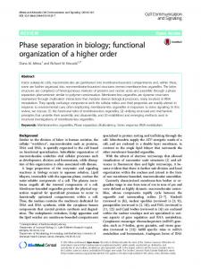
FIG. 4. Snapshots of the phase separation in 2D at the time when the QI almost reaches the left boundary. Straight QI 共5兲 for ⑀ = 1, 具u典 = 0.1, v = 0.05 共a兲. Modulated QI 共15兲 for ⑀ = 1, a = 4, p = ␲ / 16: 具u典 = 0 and v = 0.01 共b兲, v = 0.055, 共c兲, 具u典 = 0.1, v = 0.1 共d兲.

nisms. In particular, for the relevant off-critical case a noise strength ␦u ⬎ 具u典, violating the Ginzburg criterion, was chosen 关21兴. Consequently, for instance, the change of the domain orientation from perpendicular to parallel with increasing v reported in 关21兴 is considered as an artifact. Finally we have studied the influence of a periodic modulation of the QI which reads as follows:

⑀共x,y,t兲 =

再

− ⑀ , x ⬍ lx + a cos共py兲 − vt, + ⑀ , x ⬎ lx + a cos共py兲 − vt.

冎

共15兲

In the case of a critical quench, we found that the velocity vc at which the transition from parallel stripe patterns 关similar to Fig. 4共a兲兴 to perpendicular ones 关Fig. 4共b兲兴 occurs depends on the modulation amplitude a. This dependence is very strong for values a of the order of the typical domain size at the initial stage of phase separation 共a ⬃ ␭m = ␲ / qm兲. Furthermore, vc decreases with decreasing modulation wave number p. For p smaller than the wave number qm of the fastestgrowing mode, patterns with a cellular morphology forming behind the moving QI have been found 关Fig. 4共c兲兴. In the case of an off-critical quench, we found that 具u典 ⫽ 0 favors the formation of regular cellular planforms 关Fig. 4共d兲兴 at intermediate QI velocities, in analogy to the transition from parallel to perpendicular stripes for 具u典 = 0. As a main result of the paper, we have demonstrated that directional quenching in the CH model leads to the formation

关1兴 J. D. Gunton, M. San Miguel, and P. S. Sahni, in Phase Transitions and Critical Phenomena, edited by C. Domb and J. L. Lebowitz 共Academic, London, 1983兲, Vol. 8. 关2兴 A. J. Bray, Adv. Phys. 43, 357 共1994兲. 关3兴 M. C. Cross and P. C. Hohenberg, Rev. Mod. Phys. 65, 851 共1993兲. 关4兴 J. Vörös, T. Blättler, and M. Textor, MRS Bull. 30, 202 共2005兲. 关5兴 H. Sirringhaus, Adv. Mater. 共Weinheim, Ger.兲 17, 2411 共2005兲. 关6兴 D. C. Coffey and D. S. Ginger, J. Am. Chem. Soc. 127, 4564 共2005兲. 关7兴 G. Fichet, N. Corcoran, P. K. H. Ho, A. C. Arias, J. D. MacKenzie, W. T. S. Huck, and R. H. Friend, Adv. Mater. 共Weinheim, Ger.兲 16, 1908 共2004兲. 关8兴 H. Tanaka and T. Sigehuzi, Phys. Rev. Lett. 75, 874 共1995兲. 关9兴 C. L. Emmott and A. J. Bray, Phys. Rev. E 54, 4568 共1996兲. 关10兴 L. Berthier, Phys. Rev. E 63, 051503 共2001兲. 关11兴 A. A. Golovin, A. A. Nepomnyashchy, S. H. Davis, and M. A. Zaks, Phys. Rev. Lett. 86, 1550 共2001兲. 关12兴 A. Voit, A. Krekhov, W. Enge, L. Kramer, and W. Köhler, Phys. Rev. Lett. 94, 214501 共2005兲. 关13兴 A. P. Krekhov and L. Kramer, Phys. Rev. E 70, 061801

of periodic solutions with the wavelength uniquely selected by the velocity of the quench interface. This is in contrast to Ginzburg-Landau models with a nonconserved order parameter where a moving quench interface leaves no kinks behind in the wake 关24兴. The 1D CH model has recently found a new interesting application in liquid crystals to describe Ising walls between symmetry-degenerated director configurations 关25,26兴. It should be possible to verify our predictions on wavelength selection by dragging the liquid-crystal layer into a homogeneous magnetic field. In conclusion, controlling phase separation by directional quenching turns out to be a promising tool to create regular structures in material science. Although slow coarsening cannot be avoided by directional quenching in principle, longlived periodic patterns can be “frozen in”—e.g., by a deep quench, induced polymerization, chemical treatment, etc. In this respect it would be certainly rewarding to study in more depth the 2D case where interesting cellular structures have been detected and in particular the 3D case. I am deeply indebted to the late Lorenz Kramer from whom I have benefited a lot regarding the concept used in this paper. It is a pleasure to thank W. Pesch and W. Zimmermann for stimulating discussions and for critically reading the paper. Financial support by Deutsche Forschungsgemeinschaft Grant No. SFB 481 is gratefully acknowledged.

共2004兲. 关14兴 J. W. Cahn and J. E. Hilliard, J. Chem. Phys. 28, 258 共1958兲; 31, 688 共1959兲. 关15兴 P. C. Hohenberg and B. I. Halperin, Rev. Mod. Phys. 49, 435 共1977兲. 关16兴 J. S. Langer, Ann. Phys. 65, 53 共1971兲. 关17兴 T. Kawakatsu and T. Munakata, Prog. Theor. Phys. 74, 11 共1985兲. 关18兴 W. van Saarloos, Phys. Rep. 386, 29 共2003兲. 关19兴 S. Rüdiger, E. M. Nicola, J. Casademunt, and L. Kramer, Phys. Rep. 447, 73 共2007兲. 关20兴 H. Furukawa, Physica A 180, 128 共1992兲. 关21兴 B. Liu, H. Zhang, and Y. Yang, J. Chem. Phys. 113, 719 共2000兲. 关22兴 E. Ben-Jacob, H. Brand, G. Dee, L. Kramer, and J. S. Langer, Physica D 14, 348 共1985兲. 关23兴 K. Binder, J. Chem. Phys. 79, 6387 共1983兲. 关24兴 N. B. Kopnin and E. V. Thuneberg, Phys. Rev. Lett. 83, 116 共1999兲. 关25兴 C. Chevallard, M. Clerc, P. Coullet, and J.-M. Gilli, Europhys. Lett. 58, 686 共2002兲. 关26兴 T. Nagaya and J. M. Gilli, Phys. Rev. Lett. 92, 145504 共2004兲.

035302-4