FORMULATION AND OPTIMIZATION OF ROBUST SENSOR PLACEMENT PROBLEMS FOR CONTAMINANT WARNING SYSTEMS JEAN-PAUL WATSON1 WILLIAM E. HART1 REGAN MURRAY2 Sandia National Laboratories1 Albuquerque, New Mexico Environmental Protection Agency – NHSRC2 Cincinnati, Ohio
[email protected] [email protected] [email protected]
Abstract The sensor placement problem (SPP) in contaminant warning system (CWS) design for water distribution networks involves maximizing the level of protection afforded by a limited number of sensors. In existing SPP formulations, the protection level is typically quantified as either the expected impact of a contamination event, weighted by occurrence probability, or the proportion of events that are detectable. In these formulations, the issue of how to mitigate against potentially high-impact events is either handled implicitly or ignored entirely. Consequently, any solutions of these formulations run the serious risk of failing to protect against any number of high-impact, 9/11-style attacks. This risk is further amplified by the fact that reliable estimation of contamination event probabilities is extremely difficult, such that existing SPP formulations may significantly discount the potential of high-impact events. In contrast, robust formulations of the SPP directly address these concerns by focusing strictly on a subset of high-impact contamination events, and placing sensors to minimize the impact of such events. We introduce several robust formulations of the SPP that are distinguished by how they quantify the potential damage due to high-impact contamination events. These include minimization of the worst-case impact, the Value at Risk (VaR), and the Tail-Conditional Expectation (TCE). The worst-case formulation is equivalent to the p-center problem in facility location theory. VaR and TCE are standard measures of robustness in the financial literature; the corresponding robust formulations of the SPP respectively minimize the (1-α)% largest impact and a weighted sum of the α% largest impacts. All formulations can be expressed as Mixed-Integer Programs (MIPs), which can be solved using both commercial MIP solvers and specialized heuristics. Additionally, we develop computational methods for exploring the performance trade-offs between robust and expectation-based SPP formulations. We use this framework to explore the nature of robust versus expectation-based solutions to the SPP on three real-world water distribution networks, ranging in size from 400 to over 10,000 junctions. We observe that robust SPP formulations are one or more orders of magnitude more difficult to solve than expectation-based SPPs. Our results indicate that simple heuristics yield optimal solutions to the smaller test problems in shorter run-times than MIP solvers, and yield higher-quality solutions for larger test problems. For realistic sensor budgets, solutions with low expected impact fail to protect against large numbers of high-impact contamination events (with impact 5-10 times larger than the expectation). In contrast, we show that solutions to robust SPPs yield 10-25number and magnitude of high-impact events. In general, our results indicate that it is possible to trade off mean impact versus high impact performance 1
in real-world water distribution networks, exposing a key, unexplored dimension in the design of sensor placements for CWSs. Further analysis indicates that the performance of solutions to the worst-case, VaR, and TCE formulations is strongly correlated. Consequently, it may be possible in the future to restrict focus to the worst-case robust SPP formulation, which is significantly easier to solve than the VaR and TCE variants.
Keywords Sensor Placement, Contaminant Warning System Design, Robust Optimization.
1 Introduction Algorithmic methods for placing sensors to support the design of Contaminant Warning Systems (CWSs) for municipal water distribution networks have received significant attention from researchers and practitioners over the last five to ten years (Kessler et al., 1998; Ostfeld and Salomons, 2004; Berry et al., 2005a, 2006b). Without exception, these algorithms attempt to either minimize the expected impact of a contamination event or maximize the proportion of contamination events that are ultimately detected, independent of impact. Recently, Watson et al. (2004) showed that the two formulations are in fact identical, as the second formulation can be expressed in terms of the first. In the canonical formulation, contamination event probabilities are either assumed to be uniform, or are estimated based on factors such as the difficulty of accessing a particular component of a distribution network. Given a broad range of contamination scenarios, sensor placement algorithms attempt to minimize the probability-weighted sum of contamination event impact, i.e., the expected impact. The most advanced algorithms currently available can successfully generate provably optimal sensor placements to very large (e.g., 10,000+ junction) distribution networks for very large numbers (e.g., 50,000+ ) of possible scenarios, in minutes to hours of CPU time on a modern workstation (Berry et al., 2006b). Consequently, the basic sensor placement problem for CWS design is effectively solved for most practical networks, and the research emphasis has moved toward integration of more realistic modeling assumptions such as imperfect sensors (Berry et al., 2006a), installation cost and accessibility considerations (Berry et al., 2005b), and significantly larger numbers of possible contamination scenarios. One currently unexplored and potentially key aspect of the sensor placement optimization problem involves formulations in which the design objective is not minimization of the expected impact, but rather minimization of worst-case impact or other “robust” measures that focus strictly on high-consequence contamination events. The lack of research into these alternative formulations is perhaps counterintuitive in a post-9/11 environment, although it is worth noting that the US Environmental Protection Agency (EPA) has no specific tasking to investigate CWS security measures that mitigate strictly against the highest-impact contamination events. However, in our working experience with various US water municipalities, a common reaction when discussing expectation-based formulations of the sensor placement optimization problem is “Why not only concentrate on high-impact contamination events?”. From a practical standpoint, even optimal expectation-based solutions can permit numerous high-impact contamination events (e.g., as discussed below in Section 2). Further, accurate estimation of event probabilities is notoriously difficult, allowing for optimistic de-emphasis of high-impact events. Although the final determination of the design objective ultimately rests with policy-makers at various levels, the aforementioned factors strongly suggest that, at a minimum, there is a need to understand the differences between and implications of both expectation-based and robust sensor placements. In this paper, we introduce a number of robust impact measures of sensor placement performance, drawing heavily from existing literature on robust optimization from the financial community. Using both exact mixed-integer programming methods and heuristic alternatives, we identify optimal and presumed-optimal 2
sensor placements that minimize these robust impact measures on three real-world water distribution networks. We find that, as anticipated, sensor placements that minimize the expected impact admit – without exception – a non-trivial number of very high-impact contamination events. These high-impact events can be mitigated with robust sensor placements, e.g., we observe that significant reductions in the worst-case impact are possible. These reductions come at the necessary expense of an increase in the mean impact of a contamination event. However, the degree to which trade-offs are possible is significantly larger than anticipated, to the point where the performance discrepancies are so large that it is likely to impact the higher-level CWS design process. This analysis is not without cost, as robust sensor placements are significantly more difficult to compute than their expected-case counterparts. Specifically, mixed-integer programming formulations can fail to converge on robust formulations even after days of CPU time. Fortunately, heuristic methods can yield high-quality solutions in hours or less of CPU time, although we are currently unable to establish optimality in all instances. Finally, different robust measures appear highly correlated, such that minimization of one measure provides optimal or near-optimal solutions with respect to other robust measures. The remainder of this paper is organized as follows. We begin in Section 2 with a motivating example to concretely and in detail illustrate differences in the characteristics of sensor placements that are optimal with respect to expectation-based and worst-case performance. Various robust impact measures are then introduced in Section 3. Section 4 details the test networks, contamination event scenarios, and problem formulation that we use in the analysis discussed in Section 5; the latter details qualitative and quantitative differences between optimal expectation-based and robust sensor placements. We defer discussion of the specific algorithms used in this analysis to Section 6, which also addresses the computational difficulty of robust sensor placement formulations. Finally, we conclude in Section 7 with a discussion of the implications of our results.
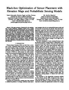
2 Motivating Example To concretely illustrate the issues involving relative trade-offs between expected-case and robust sensor placement, we begin with an example from a real-world distribution network. The network is simply denoted Network2; this and other test networks are described in detail subsequently in Section 4. Using the experimental methodology (Section 4) and algorithms (Section 6) presented below, we determine sensor placements for Network2 – given a budget of 20 sensors – that respectively minimize the expected-case and worst-case impact of a contamination event. The precise details of the contamination scenarios are documented in Section 4; impact is quantified as the number of people sickened by a contamination event. Histograms of the impact of a range of contamination events (in this case, injections at each junction with non-zero demand, for a total of 1,621 events) given the optimal expected-case and worst-case sensor placements are shown in Figure 1. We first consider the distribution of impacts given an optimal expected-case sensor placement, as shown in the left side of Figure 1. The mean and worst-case impacts of a contamination event given this sensor placement are 685 and 4,902, respectively. The distribution exhibits a key feature of sensor placements that minimize the expected-case: the presence of non-trivial numbers of events that yield impacts up to nearly ten times greater than that of the mean. Specifically, eight contamination events yield impacts greater than 4,000 individuals sickened, while an additional six contamination events yields impacts between 3,500 and 4,000 individuals sickened. Next, we consider the distribution of impacts given a sensor placement that minimizes the worst-case impact of a contamination event, as shown in the right side of Figure 1. In contrasting the two distributions, we immediately observe a significant reduction in the density of very high-impact contamination events. In particular, the highest-impact event sickens 3,490 individuals, in contrast to 4,902 individuals under the optimal expected-case sensor placement; clearly, all 14 of the highest-impact events in the expected-case
3
400
350
350
300
300
250
250 Frequency
Frequency
400
200
200
150
150
100
100
50
50
0
0
1000
2000 3000 Population Sickened
4000
0
5000
0
1000
2000 3000 Population Sickened
4000
5000
Figure 1: Histograms of the (quantity of) population sickened for various contamination events under optimal expected-case (left figure) and worst-case (right figure) sensor placements. scenario are mitigated by a sensor placement that minimizes the worst case. However, as is expected, the reduction of high-impact events increases the number of small-to-moderate impact events. The worst-case sensor placement yields a mean impact of 882 individuals sickened, representing a 29% increase relative to the expected-case sensor placement. Even more dramatic growth is observed in the upper quartile impact, from 1,011 under the expected-case sensor placement to 1,445 under the worst-case sensor placement (representing a 43% increase). The question for decision-makers in water security management is then: Is a large (in this case 29%) reduction in the worst-case impact worth the corresponding increase in the mean and moderate case? Both adversarial and engineering factors dictate the answer to this question. Although very high-impact contamination events typically represent a small fraction of the total number of possible contamination events, they are not a priori any more difficult to realize. For example, backflow injections can be carried out with roughly equiprobable success at any node in a typical network. Further, contamination event probabilities are notoriously difficult to accurately quantify, due to a variety of estimates that must be made with respect to adversarial intent, capability, and level of target vulnerability. Reliance on estimated event probabilities is therefore not without potentially significant risk; de-emphasis of high-impact injections with perceived low probability of occurrence may cause sensors to be placed in regions of the network that allow many worst- or near-worst-case events to proceed unmitigated. Finally, adversarial characteristics have a significant impact on the design and assessment of a sensor placement. Intelligent and informed adversaries are likely to identify and initiate those injection events that yield the highest-consequence impacts. Although some measures can be taken to mitigate intelligent adversaries, e.g., security classification of network structure and flow characteristics so that impacts cannot be predicted, they do not guarantee protection; insiders will always remain a threat, and trained engineers may be able to infer such characteristics from external observation with sufficient accuracy. Consequently, a rational alternative to estimating contamination event probabilities is to simply assume an omniscient adversary and focus on protecting against the worst-case scenarios.
4
3 Quantifying Solution Robustness Informally, “robust” optimization methods focus on generating solutions that minimize down-side risk. The majority of early research on robust optimization originated in the financial academic community. Clearly, quantification of solution robustness is a key component of any robust optimization method. Two primary measures of solution robustness can be found in the body of financial literature: Value-at-Risk (VaR) and Conditional Value-at-Risk (CVaR). Given a set of potential scenarios and their associated costs (e.g., impact to the population in the context of sensor placement), VaR is defined as the cost of the 1 − α most costly scenario (Holton, 2003). Typically, α is taken as 0.05, such that minimization of VaR effectively allows an optimization algorithm to ignore any costs associated with the top α fraction of scenarios. VaR is an international standard for risk quantification in the banking community, and has seen widespread application in related contexts. In contrast to VaR, CVaR quantifies the total cost of the α most costly scenarios (Artzner et al., 1999); again, α is typically taken as 0.05. Consequently, algorithms that minimize CVaR must make decisions in order to reduce the α-most “tail mass” of the cost distribution. CVaR is closely related the concept of Tail-Conditional Expectation (TCE), which quantifies the cost expectation over the α most costly scenarios. In the case of continuous cost distributions, CVaR = TCE. In the case of discrete cost distributions, CVaR is a continuous approximation to the true cost distribution, such that TCE < CVaR. Finally, we additionally consider perhaps the most intuitive measure of down-side risk, that of the worst case cost, which we denote simply as Worst. Overall, we observe that these four risk or robustness measures are related through the following inequality: VaR ≤ CVaR ≤ TCE ≤ Worst.
4 Test Networks and Problem Formulation We now describe the test networks (Section 4.1), experimental methodology (Section 4.1), and problem formulations (Section 4.2) used to support the motivating analysis presented previously in Section 2 and the more comprehensive analysis presented subsequently in Section 5.
4.1 Networks and Contamination Scenarios We report computational results for three real, large-scale municipal water distribution networks. The networks are denoted simply as Network1, Network2, and Network3; the identities of the corresponding municipalities are withheld due to security concerns. Network1 consists of roughly 400 junctions, 500 pipes, and a small number of tanks and reservoirs. Network2 consists of roughly 3000 junctions, 4000 pipes, and roughly 50 tanks and reservoirs. Network3 consists of roughly 12000 junctions, 14000 pipes, and a handful of reservoirs; there are no tanks or well sources in this municipality. All of the models are skeletonized, although the degree of skeletonization in Network1 and Network2 is much greater than in Network3. Graphical representations of Network1, Network2, and Network3 are respectively shown in the upper left, upper right, and lower portion of Figure 2. Each figure was produced by manually “morphing” or altering (e.g., through pipe lengthening or coordinate translation/rotation) key topological features of the original network structure to further inhibit identification of the source municipality. Local topologies were largely preserved in this process, such that the graphics faithfully capture the overall characteristics of the underlying network structures. Sanitized versions of all three networks, in the form of EPANET input files, are available from the authors. While these files contain no coordinate information, all data other than that relating to labels (which have been anonymized) are unaltered. Consequently, all computed hydraulic and water quality information accurately reflect (within the fidelity limits of the data and the computational model) the dynamics of the source municipality. Our goals in making these files available to the broader research community are to facilitate independent replication of our results and to introduce larger, more realistic networks into the currently limited suite of available test problems. 5
Figure 2: Graphical depiction of Network1 (upper left), Network2 (upper right), and Network3 (lower) topologies. See text for details. Network hydraulics are simulated over a 96 hour duration, representing multiple iterations of a typical daily demand cycle. For each junction with non-zero demand, a single contamination scenario is defined. Each scenario starts at time t = 0 and continues for a duration of 12 hours. Scenarios are modeled as biological mass injections with a constant rate of 5.78e+10 organisms per minute. We note that the p-median formulation, via the dsj , allows for the use of arbitrarily complex contamination scenarios, e.g., multiple simultaneous injection sites with different contaminants at variable injection strengths and durations. We assume uniform scenario probabilities, such that all results are normalized by the number of non-zero demand junctions to obtain an expectation. Water quality simulations are performed for each scenario, with a time-step resolution of 5 minutes. The resulting τsj are then used to compute the impact parameters dsj for the various design objectives All hydraulic and water quality simulations are performed using EPANET (Rossman, 1999).
4.2 Formulation To determine an optimal sensor placement P and the corresponding minimal x, we formulate the p-median problem as a mixed-integer (linear) program (MIP), which we then solve using a commercially available MIP solver. The MIP-related terms used throughout this paper are defined in the Mathematical Programming Glossary (Greenberg, 2006). A MIP formulation of the p-median problem is given as follows: 6
Minimize
X X
dsj xsj
(1)
s∈S j∈L∪{q}
Subject to
X
xsj = 1
∀s ∈ S
(2)
∀j ∈ L
(3)
j∈L∪{q}
xsj ≤ yj X yj = p
(4)
j∈L
yj ∈ {0, 1}
∀j ∈ L
(5)
0 ≤ xsj ≤ 1
∀s ∈ S, j ∈ L ∪ {q}
(6)
The binary yj variables determine whether a sensor is placed at a junction j ∈ L. Linearization of Equation 1 is achieved through the introduction of auxiliary variables xsj , which indicate whether a sensor placed at junction j is the first to detect scenario s. Constraint 3 ensures that detection is possible only if a sensor exists at junction j. The xsj variables are implicitly binary due to a combination of binary yj , Constraint 3, and the objective function pressure induced by Equation 1. Constraint 2 guarantees that each scenario s ∈ S is first detected by exactly one sensor, either at q or in the set L; ties are broken arbitrarily. Finally, the objective function (Equation 1) ensures that detection of a scenario s is assigned to the junction j ∈ L ∪ {q} such that dsj is minimal. The impact of a potential contamination scenario is determined via transport simulation. Specifically, EPANET (Rossman, 1999) is used to generate a time-series τsj of contaminant concentration at each junction j ∈ L for each scenario s ∈ S. The resulting time-series are then used to compute the network-wide impact dsj of the scenario s assuming first detection via a sensor placed at junction j. More formally, let γsj denote the earliest time t at which a sensor at junction j can detect contaminant due to scenario s, e.g., when contaminant concentration reaches a specific detection threshold. If contaminant from scenario s fails to reach junction j, then γsj = t∗ , where t∗ denotes either the end of the simulation or an appropriate user-specified delay; otherwise, γsj can easily be computed from τsj . Next, we define dsj = ds (γsj ), i.e., the aggregate, network-wide damage incurred if scenario s is first detected at time γsj . In our analysis, dsq = ds (t∗ ). We assume without loss of generality that a sensor placed at a junction j ∈ L is capable of immediately detecting any scenario s ∈ S at j once non-zero concentration levels of a contaminant are present. Finally, in the absence of realistic alarm procedures and mitigation strategies, we assume that both consumption and propagation of contaminant is terminated once detection occurs. Population Exposed (pe): This objective quantifies the number of people sickened by exposure to the injected contaminant, as defined by the demand-based model described in Murray et al. (2006). Specific values for the numerous parameters in the dosage-response computation can be obtained from the authors. Alternative models of population exposure have assumed the availability of population estimates on a perjunction basis (Berry et al., 2005a; Watson et al., 2004). While correcting the obvious deficiency of demandbased models, reliable estimates of population density are generally unavailable.
5 Expectation versus Robust Sensor Placements We now examine the differences between expectation-based and robust sensor placement performance in detail. The analysis is broken into two components. Specifically, we expand the analysis presented in Section 2 to robustness measures other than Worst, in addition to Network1 and Network3. For each of our test networks, we use the heuristic algorithm described below in Section 6 to develop disparate sensor placements that attempt to minimize both Mean and the various robust performance metrics. 7
Objective to Minimize Mean VaR TCE Worst
Mean 143.37 174.69 189.82 161.64
Performance Metric VaR TCE Worst 476.35 749.26 1248.51 388.25 824.39 1446.62 476.35 539.19 678.85 564.72 586.83 604.59
Table 1: Performance of expectation-based and robust sensor placements in terms of various metrics for Network1. The placements consist of 5 sensors mitigating against 105 possible contamination events.
Objective to Minimize Mean VaR TCE Worst
Mean 685.41 740.04 757.30 869.22
Performance Metric VaR TCE 2244.32 2953.46 2018.84 2699.41 2112.42 2507.61 2772.83 2990.19
Worst 4901.74 5076.31 3961.72 3489.73
Table 2: Performance of expectation-based and robust sensor placements in terms of various metrics for Network2. The placements consist of 20 sensors mitigating against 1621 possible contamination events.
Objective to Minimize Mean VaR TCE Worst
Mean 319.96 334.76 342.63 463.38
Performance Metric VaR TCE 1214.05 1767.32 1187.67 1780.8 1283.37 1684.54 1934.32 2315.16
Worst 4779.72 5793.52 4219.39 3079.47
Table 3: Performance of expectation-based and robust sensor placements in terms of various metrics for Network3. The placements consist of 20 sensors mitigating against 9705 possible contamination events. As discussed in Section 6, we cannot in general guarantee the optimality of the robust sensor placements due to the marked increase in difficulty of the corresponding facility location MIP formulations relative to the baseline expectation-based variant. The performance of each of the resulting sensor placements is then quantified in terms of the Mean, VaR, TCE, and Worst metrics. The results for Network1 through Network3 are respectively shown in Tables 1 through 3. We observe that in each of the tables, the inequality VaR ≤ CVaR ≤ TCE ≤ Worst holds, as required, for both the diagonal entries and the entries of each row. We first consider the results for Network1 (Table 1), in which 5 sensors are placed to mitigate against contamination events initiated at each of the 105 junctions with non-zero demand. Due to the small scale of this problem, we are able to establish the optimality of the Worst sensor placement. Relative to the example shown in Section 2, we observe even more dramatic differences between the Mean and Worst sensor placements: the worst-case impact can be cut in half for less than a 13% increase in the mean impact. Via exhaustive, implicit enumeration of the solution space via a modified MIP branch-and-bound procedure, we determined that there are in fact a number of alternative global optima that satisfy Worst = 604.59. This observation raises the possibility that solutions with Worst = 604.59 and Mean ≤ 161.64 may exist. Indeed, using a modified version of our heuristic algorithm that allow specification of side constraints, we found such a solution with Worst = 604.59 and Mean = 147.93; the latter represents slightly larger than a 3% increase relative to the optimal value of Mean = 143.37. Although we could in principle perform a similar analysis for each of the results shown in Tables 1 through 3, side constraints further increase the difficulty of the
8
robust problem formulation, which as indicated in Section 6 is already substantial. Rather, we simply note that optimality (or presumed optimality) with respect to one measure does guarantee conditional optimality on the complementary measures, due to the potential presence of alternative optima. Finally, we observe that although the performance of the Mean and Worst placements is significantly different, the placements themselves are not; both of the em Worst placements discussed above share sensors at respectively two and three of the possible five junctions. Given that VaR, TCE, and WorsT all quantify related aspects of the distribution of high-impact contamination events, we expected a priori that sensor placements minimizing these robustness measures would be strongly correlated in terms of their performance. Unexpectedly, the data shown in Table 1 indicate this is not the case. For example, the Worst performance of the VaR-optimal solution is more than double than of the optimal Worst performance. Even discounting potential effects due to alternative global optima, the effect remains significant; minimizing Worst subject to VaR ≤ 388.25 yields only a slight reduction to Worst = 1248.51. Similar discrepancies exist between the observed and optimal values of TCE given a VaR-optimal placement. Of course, minimization of VaR allows for any distribution of the remaining α proportion of high-impact events, so the results are consistent. However, the degree of the divergence was unexpected. In general, this behavior simply reinforces the importance of understanding and analyzing the performance metrics used in optimization; apparently subtle differences (e.g., between TCE and Worst) in even the subset of robust metrics can yield significant differences in sensor configurations and performance. Next, we consider the results for Network2 (Table 2), which extends the analysis presented in Section 2 to other robust metrics. Expanding on the previously noted observation that trade-offs in Mean and Worst performance that are possible, we again observe alternative optima in this problem for the Worst-optimal performance. Mirroring the approach discussed above for Network1, we were able to generate a solution via imposition of side constraints with Worst = 3489.73 and Mean = 768.16 – in contrast to the initial value of Mean = 869.22 given the Worst-optimal solution. Consequently, it is possible in Network2 obtain a nearly 30% reduction in worst-case impact at the expense of a relatively minor 12% increase in mean impact. Interestingly, despite the similar performance, this solution and the Mean-optimal solution share sensors at only two of the possible twenty junctions in common. Finally, as with the results for Network1, the performance of the robust metrics is not strongly correlated – even accounting for the presence of alternative global optima.
6 Algorithms and Computational Experience We have previously described both heuristic and exact algorithms for solving expectation-based facility location formulations of the SPP, i.e., the p-median problem (Berry et al., 2006b). We employed commercially available MIP solvers, specifically ILOG’s CPLEX 9.1 and 10.0 packages1 , to compute provably optimal solutions to the p-median MIP formulation described in Section 4.2. Using various modeling techniques to reduce the size of the basic formulation, we were able to identify optimal solutions to Network3 in roughly 15 minutes of CPU time on a modern workstation. These techniques take advantage of equality in the arrival time of contaminant at various junctions, due to the imposition of a discretized water quality time-step. Consequently, the impacts dsj are identical for various j, and the j can be collected into “superfacilities”, thereby reducing the effective size of the p-median problem. We also applied a Greedy Randomized Adaptive Search Procedure (GRASP) to heuristically generate high-quality solutions to the p-median MIP formulation. The algorithm, fully described in Resende and Werneck (2004), is a simple multi-start local search procedure in which steepest-descent hill-climbing is applied to a number N of initial solutions. The neighborhood used in the GRASP algorithm is based on facility exchange: each move consists of closing a currently opened facility and opening a currently closed 1
http://www.ilog.com
9
Objective to Minimize Mean Worst VaR TCE
Mean Run-Time per Local Optimum Network1 Network2 Network3 0.01s 0.81s 6.5s 0.02s 97s 4.4hrs 0.05s 643s 20.4hrs 0.06s 810s 26.0hrs
Table 4: Mean run-times required for the GRASP heuristic to generate a local optimum to both expectationbased and robust variants of the sensor placement problem, for each of our test networks.
Objective to Minimize Mean Worst CVaR
Network1 0.70s 8m20s 3m18s
Run-Time Network2 3m2s >24hrs >24hrs
Network3 47m31s >48hrs >96hrs
Table 5: Run-times to solve the exact MIP models for expectation-based and robust variants of the sensor placement problem, for each of our test problems. facility. The hill-climbing procedure selects the move that results in the largest decrease in solution cost at each iteration, and terminates once no improvements are possible. The best of the N solutions is returned by the algorithm. Our experiments indicate that the GRASP heuristic obtains solutions faster than the MIP solves described above, e.g., in under three minutes for Network3. Further, in all cases investigated, the obtained solutions were optimal, i.e., equivalent in quality to those obtained by CPLEX. To facilitate the present analysis, we extended the GRASP heuristic to enable solution of the robust variants of the facility formulation described in Section 4.2. The extensions involved modification of the move evaluation code that determines the change in solution cost associated with simultaneously closing a facility x and opening a facility y. The efficiency of the resulting algorithm is dictated by the speed of move evaluation, which can be accelerated by various analytic results specific to the p-center and related facility location problems; we defer to Mladenovic et al. (2003) for a discussion of these techniques. As hinted at previously, robust formulations of the SPP are empirically much more difficult than their expectation-based counterparts. To quantify this discrepancy, we consider the average run-times required to generate a single sample, i.e., a local optimum, under each of the Mean, VaR, TCE, and Worst metrics. Our computational platform is a workstation containing 64-bit AMD 2.2GHz Opteron central processors running under the Linux 2.6 operating system; the platform possess 64GB of RAM, such that run-time issues relating to memory paging are non-existent. All codes were written in C++ and compiled under gcc 3.4.3 with level 2 optimization. The results for all three of our test networks are shown in Table 4, using the sensor budgets indicated in Section 4.1. The run-times include the time required to load the problem instance. The results clearly illustrate the difficulty of robust variants of the SPP. Although Network1 run-times are clearly negligible for any metric, the divergence between the Mean and other metrics is significant for Network2; the run-times under the Mean and Worst metrics differ by a factor of 100, and is even larger under the VaR and TCE metrics. Relative to Network1, the growth in difficulty is accentuated in part due to the growth in the sensor budget p, as the number of moves available from any solution is a monotonically increasing function of both m and p for the range of p we consider. Even larger analogous discrepancies are observed on Network3, where the run-times under the Mean and Worst differ by a factor of nearly 40. The difficulty of computing samples for the VaR and TCE metrics is even more difficult than for Worst. This is due to the additional need, relative to the Worst computation, for sorting the impacts (in the case of VaR and TCE) and computing the tail expectation (in the case of TCE). 10
We have also investigated extensions of our basic MIP model (Berry et al., 2006b) to robust optimization metrics. To generate a MIP formulation to minimize Worst performance, we simply replace Equation 1 with the following: X dsj xsj (7) minimize maxs∈S j∈L∪{q}
The extended formulation for minimization of CVaR (the continuous approximation to TCE, which in general is discretized) is significantly more complicated, and is not discussed herein. We used CPLEX 10.0, a state-of-the-art commercial MIP solver, to minimize Mean, CVaR, and Worst for each of our test networks. The computational platform was identical to that described above for the heuristic tests, and a limit of 24 hours was imposed on each individual run. The results are reported in Table 5. We first consider the results for Network1, which are analogous to those reported for the heuristic in Table 4. Specifically, minimization of the robust metrics requires several orders of magnitude more run-time than required for the Mean metric. However, minimization of CVaR is less costly than Worst; we currently have no explanation for this discrepancy. Next, we examine the results for Network2 and Network3. In no case could CPLEX minimize the robust metrics within the allocated time limit of 24 hours. Overall, these results clearly reinforce the dramatic differences in difficulty involved in minimization of expectation-based versus robust performance metrics; the latter require at least 20 times more computational effort, and in most cases, significantly more. From a practical standpoint, this currently prevents us from establishing proofs of optimality for heuristic solutions for all but the smallest test networks. Overall, the data presented in Tables 4 and 5 illustrate the challenges associated with optimization of robust performance metrics. Although exact methods are tractable in the case of minimizing Mean impacts, optimal robust solutions - or at least proofs of optimality - are currently out of reach of exact methods. Even with heuristics, locating high-quality solutions to robust formulations requires a significant computational investment. However, even lacking optimal solutions, the fundamental conclusions presented in Section 5 still hold: it is possible to trade off expected versus robust performance. Future improvements in heuristic and exact technologies will further enhance our ability to exploit this characteristic. Finally, we observe that the relative difficulty of robust optimization is not necessarily inherent. Our results are empirical, rather than theoretical, and it is possible that additional research will expose additional techniques for improving algorithm performance, e.g., cuts in the case of MIPs or more effective move evaluators in the case of heuristics. Algorithms for minimizing the expected case, i.e., for solving the p-median formulation, have been extensively studied for decades, and only recently have these algorithms yielded results as impressive as those we report.
7 Conclusions Most extant algorithms for the sensor placement problem in water distribution networks consider minimization of the expected impact of a contamination event. However, the solutions generated by these algorithms admit a number of low-probability, very high-impact contamination events. The presence of these events, in addition to consideration of known inaccuracies in event probability estimation, should lead decision makers to at least assess the differences between solutions that minimize expected impact and those that focus strictly on high-consequence contamination events. We introduce a number of so-called robust metrics for quantifying the impact of high-consequence, e.g., tail, contamination events. Using both heuristic and exact optimization algorithms, we then contrast the performance characteristics of solutions that respectively minimize the mean and robust metrics. We show that it is possible to gain significant reductions in the number and degree of high-consequence events, at the expense of moderate increases in the mean impact of a contamination event. The existence of this trade-off should be of significant interest to decision makers response for CWS design, given inherent issues involved with event probability estimation and the implicit 11
desire to mitigate against 9/11-style attacks. Additionally, we find that performance with respect to different robust metrics is not highly correlated, further emphasizing the need to develop a deeper understanding of the relationship between solutions developed using different optimization metrics. Finally, we demonstrate that solution of robust formulations of the sensor placement problem are significantly more difficult than for their expectation-based counterpart. Although heuristics can identify high-quality solutions for robust formulations, exact methods are unable to tackle all but the smallest test networks. Further, non-trivial research effort will be required to develop truly efficient algorithms for solving, especially to optimality, robust formulations.
Acknowledgments Sandia is a multipurpose laboratory operated by Sandia Corporation, a Lockheed-Martin Company, for the United States Department of Energy under contract DE-AC04-94AL85000. This work was funded through an Interagency Agreement with the United States Environmental Protection Agency.
References Artzner, P., Delbaen, F., Eber, J., and Heath, D. (1999). Coherent measures of risk. Mathematical Finance, 9:203–228. Berry, J., Carr, R., Hart, W., Leung, V., Phillips, C., and Watson, J. (2006a). On the placement of imperfect sensors in municipal water networks. In Proceedings of the 8th Symposium on Water Distribution Systems Analysis. Berry, J., Fleischer, L., Hart, W., Phillips, C., and Watson, J. (2005a). Sensor placement in municipal water networks. Journal of Water Resources Planning and Management, 131(3). Berry, J., Hart, W., Phillips, C., Uber, J., and Walski, T. (2005b). Water quality sensor placement in water networks with budget constraints. In Proceedings of the ASCE/EWRI Congress. Berry, J., Hart, W., Phillips, C., Uber, J., and Watson, J. (2006b). Sensor placement in municipal water networks with temporal integer programming models. Journal of Water Resources Planning and Management: Special Issue on Drinking Water Distribution Systems Security (To Appear). Greenberg, H. (1996–2006). Mathematical Programming Glossary. World Wide Web, http://www. cudenver.edu/∼hgreenbe/glossary/. Holton, G. A. (2003). Value-at-Risk: Theory and Practice. Academic Press. Kessler, A., Ostfeld, A., and Sinai, G. (1998). Detecting accidental contaminations in municipal water networks. Journal of Water Resources Planning and Management, 124(4):192–198. Mladenovic, N., Labbe, M., and Hansen, P. (2003). Solving the p-center problem with tabu search and variable neighborhood search. Networks, 42(1):48–64. Murray, R., Uber, J., and Janke, R. (2006). Modeling acute health impacts resulting from ingestion of contaminated drinking water. Journal of Water Resources Planning and Management: Special Issue on Drinking Water Distribution Systems Security (To Appear). Ostfeld, A. and Salomons, E. (2004). Optimal layout of early warning detection stations for water distribution systems security. Journal of Water Resources Planning and Management, 130(5):377–385. 12
Resende, M. and Werneck, R. (2004). A hybrid heuristic for the p-median problem. Journal of Heuristics, 10(1):59–88. Rossman, L. (1999). The EPANET programmer’s toolkit for analysis of water distribution systems. In Proc. of the Annual Water Resources Planning and Management Conference. Watson, J., Greenberg, H., and Hart, W. (2004). A multiple-objective analysis of sensor placement optimization in water networks. In Proceedings of the ASCE/EWRI Congress.
13