Fortran codes for computing the discrete Helmholtz ... - Springer Link

Advances in Computational Mathematics 9 (1998) 391–409

391

Software Note

Fortran codes for computing the discrete Helmholtz integral operators S.M. Kirkup Integrated Sound Software, 25 Smithwell Lane, Heptonstall, Hebden Bridge HX7 7NX, UK www.soundsoft.demon.co.uk

Received November 1995; revised February 1998 Communicated by I. Sloan

In this paper Fortran subroutines for the evaluation of the discrete form of the Helmholtz integral operators Lk , Mk , Mkt and Nk for two-dimensional, three-dimensional and threedimensional axisymmetric problems are described. The subroutines are useful in the solution of Helmholtz problems via boundary element and related methods. The subroutines have been designed to be easy to use, reliable and efficient. The subroutines are also flexible in that the quadrature rule is defined as a parameter and the library functions (such as the Hankel, exponential and square root functions) are called from external routines. The subroutines are demonstrated on test problems arising from the solution of the Neumann problem exterior to a closed boundary via the Burton and Miller equation.

1.

Introduction

The Fortran subroutines described in this paper are useful in the implementation of integral equation methods for the solution of the general two-dimensional, the general three-dimensional and the axisymmetric three-dimensional Helmholtz equation, ∇2 ϕ(p) + k2 ϕ(p) = 0,

(1)

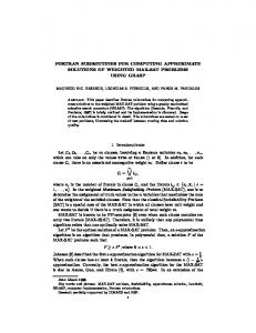
which governs ϕ(p) in a given domain and k is a complex number. The subroutines compute the discrete form of the integral operators Lk , Mk , Mkt and Nk that arise in the application of collocation to integral equation formulations of the Helmholtz equation. Expressions for the discrete integral operators are derived by approximating the boundaries by the most simple elements for each of the three cases – straight line elements for the general two-dimensional case, flat triangular elements for the general three-dimensional case and conical elements for the axisymmetric three-dimensional case – and approximating the boundary functions by a constant on each element. The elements are illustrated in figure 1. The Helmholtz integral operators are defined as follows: Z (2) {Lk µ}Γ (p) ≡ Gk (p, q)µ(q) dSq , Γ

 J.C. Baltzer AG, Science Publishers

392

S.M. Kirkup / Fortran codes for computing the discrete Helmholtz integral operators

Figure 1. The straight line, planar triangle and truncated cone elements.

Z

∂Gk (p, q)µ(q) dSq , Γ ∂nq Z  t ∂ Gk (p, q)µ(q) dSq , Mk µ Γ (p; vp ) ≡ ∂vp Γ Z ∂ ∂Gk (p, q)µ(q) dSq , {Nk µ}Γ (p; vp ) ≡ ∂vp Γ ∂nq {Mk µ}Γ (p) ≡

(3) (4) (5)

where Γ is a boundary (not necessarily closed), nq is the unique unit normal vector to Γ at q, vp is a unit directional vector passing through p and µ(q) is a function defined for q ∈ Γ. Gk (p, q) is the free-space Green’s function for the Helmholtz equation. In this paper the Green’s functions are i (6) Gk (p, q) = H0(1) (kr) (k ∈ C\{0}) in two dimensions, 4 1 eikr (k ∈ C) in three dimensions, (7) Gk (p, q) = 4π r where r = |r|, r = p − q, C is the set of complex numbers and i is the unit imaginary number. The function H0(1) is the spherical Hankel function of the first kind of order zero. The Green’s functions (6) and (7) also satisfy the following condition at infinity, known physically as the Sommerfeld radiation condition:   ∂ϕ(p) − ikϕ(p) = 0 in two dimensions, (8) lim r 1/2 r→∞ ∂r   ∂ϕ(p) lim r − ikϕ(p) = 0 in three dimensions. (9) r→∞ ∂r For the special case when k = 0 the Helmholtz equation (1) is the Laplace equation. In this particular case the chosen Green’s functions are 1 (10) G0 (p, q) = − log r in two dimensions, 2 1 1 G0 (p, q) = in three dimensions. (11) 4π r Note that limk→0 Gk (p, q) = G0 (p, q) for the three-dimensional case but not for the two-dimensional case and that G) (p, q) for the two-dimensional case does not satisfy condition (8).

S.M. Kirkup / Fortran codes for computing the discrete Helmholtz integral operators

393

For each particular case of boundary division, the discrete form of the operators is computed using the subroutines H2LC (two-dimensional), H3LC (three-dimensional) and H3ALC (axisymmetric three-dimensional). The subroutines in this paper are thus useful for the solution of the interior or exterior Helmholtz or Laplace equation via integral equation methods; the subroutines compute the matrix elements in the linear systems of equations that arise. Each subroutine is meant to be used as a tool that will be called many times within a main program. Examples of situations where the subroutines in this paper could be useful are the problems addressed in references [1,2, 7,8,11,15–28,31,32,34,35,37–39]. The solution of Helmholtz problems is important in linear acoustics and many of the referenced papers are applied to acoustic problems. In [28] the solutions of the straightforward interior, exterior and modal acoustic problems by the boundary element method are considered. The objective of this paper is to describe the underlying methods employed in computing the discrete form of the integral operators (2)–(5), to outline the Fortran subroutines and explain how the subroutines may be utilised and to demonstrate the subroutines on the Burton and Miller equation [8]. The subroutines have been written to the Fortran77 standard and employ double-precision arithmetic. The subroutines have the identifiers H2LC, H3LC and H3ALC, for computing the discrete Helmholtz integral operators for the two-dimensional, three-dimensional and three-dimensional axisymmetric cases. The subroutines’ parameter list has the following general form: SUBROUTINE H{2 or 3 or 3A}LC( complex wavenumber point (p and the unit vector vp , if necessary), geometry of the element (vertices which define element), quadrature rule (weights and abscissae for the standard element), validation and control parameters, discrete Helmholtz integral operators (output) ). For further details on the format of the codes and how to use them the reader is referred to reference [28]. 2.

Some properties of the kernel functions

The results given in this section are extracted mainly from references [9,10,17]. In the following r = p − q and r = |r|, Gk = Gk (p, q), G0 = G0 (p, q). 2.1. Derivatives of G0 with respect to r In two dimensions we have ∂G0 1 1 =− , ∂r 2π r

(12)

394

S.M. Kirkup / Fortran codes for computing the discrete Helmholtz integral operators

1 1 ∂ 2 G0 = . 2 ∂r 2π r 2

(13)

In three dimensions we have 1 1 ∂G0 , =− ∂r 4π r 2 ∂ 2 G0 1 1 = . 2 ∂r 2π r 3

(14) (15)

2.2. Derivatives of Gk (k 6= 0) with respect to r In two dimensions we have i ∂Gk = − kH1(1) , ∂r 4

(16)

where H1(1) is the spherical Hankel function of the first kind and of order one and   ∂ 2 Gk i 2 H1(1) (1) . (17) = k − H 0 ∂r 2 4 kr In three dimensions we have eikr ∂Gk = (ikr − 1), ∂r 4πr 2
eikr ∂ 2 Gk 2 2 = r 2 − 2ikr − k . ∂r 2 4πr 3

(18) (19)

2.3. Expressions for the normal derivatives of Gk The following expressions hold in both two and three dimensions and for all k: ∂Gk ∂Gk ∂r = , ∂nq ∂r ∂nq

(20)

∂Gk ∂Gk ∂r = , ∂vp ∂r ∂vp

(21)

∂Gk ∂ 2 r ∂ 2 Gk ∂r ∂r ∂ 2 Gk = + . ∂vp ∂nq ∂r ∂vp ∂nq ∂r 2 ∂vp ∂nq

(22)

2.4. Expressions for the normal derivative of r The derivatives of r with respect vp and nq may be written as follows: r · nq ∂r , =− ∂nq r

(23)

S.M. Kirkup / Fortran codes for computing the discrete Helmholtz integral operators

r · vp ∂r , = ∂vp r   1 ∂r ∂r ∂2r . = − vp · nq + ∂vp ∂nq r ∂vp ∂nq

395

(24) (25)

2.5. Expressions for ∂ 2 G0 /(∂vp ∂nq ) The following results can be derived from the substitution of (25) and (12), (13) or (14), (15) into (22) with k = 0:   1 ∂r ∂r ∂ 2 G0 vp · nq + 2 in two dimensions, (26) = ∂vp ∂nq 2πr 2 ∂vp ∂nq   ∂G0 1 ∂r ∂r vp · nq + 3 in three dimensions. (27) = ∂vp ∂nq 4πr 3 ∂vp ∂nq 2.6. Asymptotic properties In the following results, p, q ∈ Γ, where Γ is a surface and Γ is smooth at p:

lim Gk (p, q) − G0 (p, q) = O r 0 , (28) q→p


∂Gk (p, q) = O r 0 , q→p ∂vp

(29)


∂Gk (p, q) = O r 0 , ∂np

(30)

lim

lim

q→p

 lim

q→p

3.


∂ 2 G0 1 2 ∂ 2 Gk (p, q) − (p, q) + k Gk (p, q) = O r 0 . ∂vp ∂nq ∂vp ∂nq 2

(31)

Discretization of the integral operators

In order to derive the discrete forms P of the integral operators (2)–(5), Γ is approxej . The boundary function µ is replaced e = n ∆Γ imated by a set of n elements Γ j=1 e The function is then replaced by a by its equivalent on the approximate boundary Γ. constant on each element. Thus for the Lk integral operator: n Z X  e e (p) ≈ Gk (p, q)e µ(pj ) dSq {Lk µ}Γ (p) ≈ Lk µ Γ e j=1 ∆Γj n X    = µ e(pj ) Lk ee ∆Γj (p) , j=1

(32)

396

S.M. Kirkup / Fortran codes for computing the discrete Helmholtz integral operators

where ee is the unit function. The other integral operators may be discretized in a similar way. The discrete forms are thus defined as follows: Z  (p) = Gk (p, q) dSq , (33) Lk ee ∆e Γj ∆e Γj Z  ∂Gk (p) = (p, q) dSq , (34) Mk ee ∆e Γj ∆e Γj ∂nq Z  t ∂ (p; vp ) = Gk (p, q) dSq , (35) Mk ee ∆e Γj ∂vp ∆e Γj Z  ∂Gk ∂ (p; v ) = (p, q) dSq . (36) Nk ee ∆e p Γj ∂vp ∆e Γj ∂nq The derivative operator in (35) can always be carried inside the integral. The same is ej . Thus we may true for the operator in (36) when p does not lie on the element ∆Γ write Z  t ∂Gk (p; vp ) = (p, q) dSq , (37) Mk ee ∆e Γj ∆e Γj ∂vp Z  ∂ 2 Gk ej . (p; v ) = (p, q) dSq when p ∈ / ∆Γ (38) Nk ee ∆e p Γj ∆e Γj ∂vp ∂nq ej the integrals of (33)–(36) will all be regular and hence are amenable When p ∈ / ∆Γ to standard quadrature. The same is true for the integrands of (34) and (35) when ej (though not on the edge of the element). However, the evaluation of the p ∈ ∆Γ discrete integral operators (33) and (36) generally requires special treatment when ej . p ∈ ∆Γ The special techniques applied in this paper involve “subtracting out” the singularity and evaluating the singular part and remaining regular part separately. The following results are immediate from the asymptotic properties of the kernel functions (28) and (31): Z 
 (p) = L e e (p) + G (p, q) − G (p, q) dSq , (39) Lk ee ∆e 0 0 k Γj ∆e Γj ∆e Γj   1 2 k (p; v ) = N e e (p; v ) − e e (p) L Nk ee ∆e p 0 p 0 e Γj ∆Γj ∆e Γj 2  Z  2 ∂ 2 G0 1 ∂ Gk + (p, q) − (p, q) + k2 G0 (p, q) dSq , (40) ∂vp ∂nq ∂vp ∂nq 2 ∆e Γj where, in each of (39) and (40) the explicit integral is non-singular and the remaining expressions are independent of k. Evaluation in this way requires the computation of the piecewise regular integral (amenable to standard quadrature) and the determination of the subtracted out part. In computing the explicit integrals in (39), (40), it is important to note that the integrands have discontinuous derivatives at p.

S.M. Kirkup / Fortran codes for computing the discrete Helmholtz integral operators

397

In summary, the evaluation of the integral operators requires a summation of a ej set of integrand values multiplied by quadrature weights. In the case when p ∈ ∆Γ the evaluation of the subtracted out part is also required for the Lk and Nk operators.

4.

Evaluation of the discrete forms

In this section a list of operations for computing the discrete integral operators is given. This particular programme of computation is given prominence because it needs to be executed for each quadrature point and hence it is the key to determining the computational cost of the overall method. The following computational programme is intended to be optimal. Note that it is assumed that p and vp are already set. A: B: C: D: E: F: G: H: I: J: K: L: M: N: O: P: Q: R: S: T: U:

Set q the point on the element. Set nq the unit outward normal to the element at q. Compute vp · nq . Compute r. Compute r, r 2 . Compute r 3 (in the 3D case). Compute ∂r/∂nq via (23). Compute ∂r/∂vp via (24). Compute ∂r/∂nq · ∂r/∂vp . Compute ∂ 2 r/(∂vp ∂nq ) via (25). Compute kr[k · r] and ikr[i · kr]. Compute skr[kr · kr] (in the 3D cases). Compute H [Hankel function H0(1) (kr), H1(1) (kr)] for 2D problems or E [exp(ikr)] for 3D problems. Compute Green’s function via (6) or (10) for 2D or via (7) or (11) for 3D. Multiply Lk kernel by weight and add to sum. Compute ∂Gk /∂r via (16) or (12) for 2D or via (18) or (14) for 3D. Compute value of quadrature weight multiplied by the result of operation N. Compute Mk kernel multiplied by weight and add to sum. Compute Mkt kernel multiplied by weight and add to sum. Compute ∂ 2 Gk /∂r 2 via (17) or (13) for 2D or via (19) or (15) for 3D. Multiply Nk kernel by weight and add to sum.

Apart from operations E and M, each operation can be directly costed in terms of floating-point operations. Operation E computes a square root and operation M

398

S.M. Kirkup / Fortran codes for computing the discrete Helmholtz integral operators

computes a Hankel function in two-dimensional problems and a complex exponential in three-dimensional problems. The square root and the complex exponential functions are available in most programming languages, though in some cases it could be beneficial (in terms of computational cost) not to use the standard language functions. In the two-dimensional case, operation M requires the computation of the spherical Hankel functions or log functions when k is zero. An external module is required for the evaluation of the Hankel function. In the subroutines H2LC, H3LC and H3ALC the square root function and the exponential and/or Hankel function or log functions that are evaluated at each quadrature point need to be provided as external functions with the identifiers FNSQRT, FNEXP, FNHANK and FNLOG. The freedom to define the functions externally and to choose the quadrature rule allows the user to take full control of the efficiency of the subroutines. 5.

Test problem – the Burton and Miller equation

A direct or indirect integral equation formulation of the Helmholtz equation will usually consist of some or all of the Helmholtz integral operators introduced in section 2. The solution of the Helmholtz equation (1) in the exterior E to a closed boundary S with the appropriate radiation condition can be formulated as the Burton and Miller integral equation [8] α α{Mk ϕ}S (p) − ϕ(p) + β{Nk ϕ}S (p; np ) 2    β ∂ϕ(p) ∂ϕ t ∂ϕ (p) + β Mk (p; np ) + for p ∈ S, (41) = α Lk ∂n S ∂n S 2 ∂np where S is smooth at p, α and β are complex numbers, I is the identity operator and np is the unit outward normal to S at p. The solution in E can be related to the solution on S through the following equation:   ∂ϕ (p) for p ∈ E. (42) ϕ(p) = {Mk ϕ}S (p) − Lk ∂n S Equation (41) is a useful problem with which the subroutines given in the following section can be tested as it contains all four integral operators and test solutions can easily be devised. Only the solution of the Neumann problem will be considered in this paper, that is ∂ϕ/∂nq = v(p) given for all p ∈ S. The solution of the Helmholtz problem consists of two stages. The primary stage involves the solution of the integral equation (41). This yields the solution ϕ(p) for points on S. The secondary stage involves computing the solution ϕ(p) for points in E using (42). Methods of this type, known as the Boundary Element Method (see, for example, Banerjee and Butterfield [5]), for solving the exterior Helmholtz equation have been considered in [1,2,9,10,15,17,18,20,21,28,31,32,34,37,39]. Applying collocation to (41) generally requires that the closed boundary S is replaced by an approximate boundary Se made up of a set of n elements ∆Sej (j =

S.M. Kirkup / Fortran codes for computing the discrete Helmholtz integral operators

399

1, . . . , n) in the way described in section 3. Let the points pj (j = 1, . . . , n) with pj ∈ ∆Sej be the collocation points. In this paper we consider only the approximation of the boundary functions by a constant on each element. It is helpful to adopt the following notation:  [Lk ]ij = Lk ee ∆Se (pi ), (43) j  (44) [Mk ]ij = Mk ee ∆Se (pi ), j  t  t (45) Mk ij = Mk ee ∆Se (pi ; npi ), j    Nk ij = Nk ee ∆Se (pi ; npi ), (46) j

where npi is the unit outward normal to Se at pi . This gives the four n × n matrices Lk , Mk , Mtk and Nk . The approximate boundary functions can be approximated by a vector  T µ= µ e(p1 ), . . . , µ e(pn ) . The application of collocation to the Burton and Miller equation gives the following linear systems of approximations:

   (47) α Mk − 12 I + βNk ϕ ≈ αLk + Mtk + 12 I v, where vj = v(pj ) for j = 1, . . . , n. Hence the primary stage of the boundary element method entails the solution of the following linear system of equations:
 
  b = αLk + β Mtk + 12 I v, (48) α Mk − 12 I + βNk ϕ which yields approximations ϕ bj to ϕ(pj ), for j = 1, . . . , n. The secondary stage of the boundary element method requires the calculation of e the approximation to ϕ(p) where p is a point in the approximate exterior domain E. For this the discrete forms are substituted into (42) to give ϕ(p) b =

n X    bj − Lk ee ∆Se (p)vj Mk ee ∆Se (p)ϕ j

j


e . p∈E

(49)

j=1

Note that the secondary stage requires the evaluation of only two integral operators in contrast with the primary stage which requires all four. Note also that the special evaluation techniques of subtracting out the singularity are required only for the diagonal components of the matrices in (43), (46). This latter point is a typical property of integral equation methods, the outcome of which is that the generally greater cost of evaluating the discrete forms when p lies on the element is not important when assessing the overall computational cost. Test problems can easily be devised by setting ϕ(p) = Gk (p, p∗), where p ∈ E ∪ S, p∗ ∈ D (D is the interior to S) with
∂Gk ∂ϕ (p) = p, p∗ for p ∈ S. ∂np ∂np

400

6.

S.M. Kirkup / Fortran codes for computing the discrete Helmholtz integral operators

Subroutine H2LC

In this section the Fortran subroutine H2LC is described. The subroutine computes the discrete form of the two-dimensional Helmholtz integral operators. Details of the methods employed in the subroutine are given. The subroutine is applied to the Burton and Miller integral equation for the problem where the boundary is a circle and the results are given. 6.1. Background methods The regular integrals that arise are approximated by a standard quadrature rule such as a Gauss–Legendre rule which is specified in the parameter list to the subroutines. Tables of Gauss–Legendre rules are given in Stroud and Secrest [36] and can also generated from the NAG library [33]. The non-regular integrals that arise in the formulae (39) and (40) are computed via the following methods. See Jaswon and Symm [14] and Kirkup [17] for the background to these methods. The M0 and M0t operators have regular kernels, hence the aim is to find expressions for: Z  (p) = G0 (p; q) dSq , (50) L0 ee ∆e Γ ∆e Γ Z  ∂ ∂G0 (p; n ) = (p, q) dSq , (51) N0 ee ∆e p Γ ∂vp ∆e Γ ∂nq e is a straight line element, p ∈ ∆Γ e (though not on an edge or corner of the where ∆Γ e has length a + b with q = q(x) and element). Let it be assumed that the element ∆Γ p = q(0) for x ∈ [−a, b]. This gives the following formulae for (50) and (51): 1 [a + b − a log a − b log b], (p) = L0 ee ∆e Γ 2π    1 1 1 N0 ee ∆e (p; np ) = − + . Γ 2π a b 

(52) (53)

6.2. Test problem and results The test problem consists of a boundary of a circle of unit radius, centred at the origin. The exterior solution and Neumann boundary condition are determined by a point source at (0, 0.5) and a point sink at (0, −0.5). The circle is approximated by 32 straight line elements of equal length, the vertices of the regular polygon lying on the original circle. Eight point Gauss–Legendre quadrature rules are used for all but the computation of the diagonal components of the matrices where 2 × 8 point composite Gauss–Legendre quadrature rules are used. The functions FNSQRT and FNLOG simply call the corresponding standard Fortran functions. The subroutine FNHANK was constructed through the use of NAG

S.M. Kirkup / Fortran codes for computing the discrete Helmholtz integral operators

401

Table 1a Solution for the circle with k = 0.0, α = 1, β = 0. Point

Exact solution

Computed solution

1 2 3 4 5 6 7 8

0.173161 0.160666 0.139776 0.114977 0.089028 0.063136 0.037647 0.012506

0.173408 0.160913 0.140010 0.115174 0.089176 0.063236 0.037704 0.012524

(0, 2)

0.081300

0.081008

Table 1b Solution for the circle with k = 1.0, α = 1, β = i. Point

Exact solution

Computed solution

1 2 3 4 5 6 7 8

0.204820 + 0.106145i 0.190535 + 0.102052i 0.166397 + 0.094027i 0.137368 + 0.082387i 0.106643 + 0.067589i 0.075745 + 0.050206i 0.045200 + 0.030909i 0.015018 + 0.010435i

0.210022 + 0.106022i 0.195224 + 0.101934i 0.170345 + 0.093919i 0.140541 + 0.082294i 0.109068 + 0.067513i 0.077453 + 0.050150i 0.046214 + 0.030875i 0.015355 + 0.010424i

(0, 2)

0.028905 + 0.140053i

0.028868 + 0.141126i

routines S17AEF, S17AFF, S17ACF and S17ADF and the subroutine is only suitable for real values of k. Note that routines for computing the Hankel functions for complex arguments are now available in Mark 14 of the NAG Fortran library [33]. Since the problem is symmetric about the y axis and antisymmetric about the x axis, the computed and exact solutions are listed at eight collocation points. The computed and exact solutions are also compared at the exterior point (0, 2). The wavenumbers considered are k = 0.0 (with α = 1 and β = 0) and k = 1.0 (with α = 1 and β = i). Results are given in tables 1a and 1b.

7.

Subroutine H3LC

In this section the Fortran subroutine H3LC is described. The subroutine computes the discrete form of the three-dimensional Helmholtz integral operators. Details of the background methods employed by the subroutines are given. The subroutine is applied to the Burton and Miller equation for the test problem where the boundary is a cube and results are given.

402

S.M. Kirkup / Fortran codes for computing the discrete Helmholtz integral operators

7.1. Background methods The regular integrals that arise are approximated by a quadrature rule defined on a triangle. Laursen and Gellert [30] contains a selection of Gauss–Legendre quadrature rules for the standard triangle. The non-regular integrals that arise in the formulae (41) and (42) are computed by the following methods. See Jaswon and Symm [14], Terai [37], Banerjee and Butterfield [5] and Kirkup [17] for the background to these methods. The M0 and M0t operators have regular kernels, hence the aim is to find expressions for Z  (p) = G0 (p, q) dSq , (54) L0 ee ∆e Γ ∆e Γ Z  ∂G0 ∂ (p; np ) = (p, q) dSq , (55) N0 ee ∆e Γ ∂vp ∆e Γ ∂nq e is a planar triangular element, p ∈ ∆Γ e (though not on an edge or corner where ∆Γ of the element). Let R(θ) be the distance from p to the edge of the element for θ ∈ [0, 2π], as illustrated in figure 2. The integrals (54) and (55) may be written in the form Z 2π  1 (p) = R(θ) dθ, L0 ee ∆e Γ 4π 0

Figure 2. Polar integration of the triangle.

Figure 3. Division of the planar triangle.

S.M. Kirkup / Fortran codes for computing the discrete Helmholtz integral operators

 1 (p; np ) = − N0 ee ∆e Γ 4π

Z 0

2π

403

1 dθ. R(θ)

In order to evaluate the integrals, a similar technique to that described in Guermond e is divided into three ∆1 , ∆2 and ∆3 by [13] is followed. The triangular element ∆Γ joining the point p to the vertices. The resulting triangles have the form of figure 3. After some elementary analysis, we obtain     X 1  B B+A R(0) sin B log tan − log tan , L0 ee ∆Se(p) = 4π 2 2 ∆1 ,∆2 ,∆3

X  N0 ee ∆Se(p; np ) =

∆1 ,∆2 ,∆3

1 cos(B + A) − cos B . 4π R(0) sin B

7.2. Test program and results The test problem consists of a boundary of a cube with vertices (1, 1, 1), (1, 1, −1), (1, −1, 1), (1, −1, −1), (−1, 1, 1), (−1, 1, −1), (−1, −1, 1) and (−1, −1, −1). The exterior solution and the Neumann boundary condition are determined by a point source at the centre of the cube. The cube is divided into 24 uniform triangular elements, as shown in figure 4. Seven point Gaussian quadrature rules are applied to all but the computation of the diagonal components of the matrices, where a 3 × 7 point rule is used. Solutions are sought on the boundary and at the point (0, 0, 2) at wavenumbers k = 0, 1, i, 1 + i. The values of α and β in the Burton and Miller equation (41) are set as α = 1, β = 1 for all four values of k. The functions FNSQRT and FNEXP simply call the corresponding standard Fortran functions. Since the solution is similar at each collocation point, a comparison between one exact and one computed solution is given at one surface point and the exterior point. The results are given in table 2.

Figure 4. Face of the cube divided into elements.

404

S.M. Kirkup / Fortran codes for computing the discrete Helmholtz integral operators Table 2 Solution for the cube.

8.

k

α and β

Point

Exact solution

Computed solution

0.0 0.0 1.0 1.0 1.0i 1.0i 1.0 + 1.0i 1.0 + 1.0i

α = 1, β = i α = 1, β = i α = 1, β = i α = 1, β = i α = 1, β = i α = 1, β = i α = 1, β = i α = i, β = i

Coll. Pt. (0, 0, 2) Coll. Pt. (0, 0, 2) Coll. Pt. (0, 0, 2) Coll. Pt. (0, 0, 2)

0.832050 0.500000 0.300064 + 0.776060i −0.208073 + 0.454649i 0.250145 0.067668 0.090211 + 0.233313i −0.002816 + 0.061530i

0.829128 + 0.119394i 0.535075 + 0.000003i 0.163472 + 0.840514i −0.242757 + 0.516164i 0.252107 + 0.048411i 0.068024 + 0.002300i 0.049252 + 0.246489i −0.003732 + 0.061234i

Subroutine H3ALC

In this section, the Fortran subroutine H3ALC is described. The subroutine computes the discrete form of the axisymmetric three-dimensional Helmholtz integral operators. Details of the methods employed by the subroutine are given. The subroutine is applied to the Burton and Miller equation for the test problem where the boundary is a sphere with a Neumann boundary condition and results are given. 8.1. Background methods The regular integrals that arise are approximated by a two-dimensional quadrature rule defined on a rectangle which is specified in the parameter list to the subroutine. These integrals can be approximated using a Gauss–Legendre rule in the generator and θ directions. The non-regular integrals that arise in the formula are computed by the following methods. The M0 and M0t operators have regular kernels, hence the aim is to find expressions for the following: Z  (p) = G0 (p, q) dSq , (56) L0 ee ∆e Γ ∆e Γ Z  ∂ ∂G0 (p; n ) = (p, q) dSq , (57) N0 ee ∆e p Γ ∂vp ∆e Γ ∂nq e is a conical element, p ∈ ∆Γ e (though not on an edge of the element). where ∆Γ The integral in (56) is evaluated through dividing the integral with respect to the generator direction into two parts at p and transforming the integral through changing the power of the variable, as introduced in Duffy [12] and also applied in references [3,4,17]. The resulting regular integral on both parts is computed via the quadrature rule supplied to the routine. The integral in (57) is evaluated by using the result that if the surface of integration in (57) is extended to enclose a three-dimensional volume then the integral vanishes (see [17]). As each element is a truncated right circular cone, as illustrated in figure 1, a 45◦ right circular cone is added to each flat side of the element. The

S.M. Kirkup / Fortran codes for computing the discrete Helmholtz integral operators

405

integrals over the two 45◦ cones are regular and are computed by a composite rule based on the quadrature rule supplied to the subroutine. The solution is thus equal to minus the sum of the integrals over the two 45◦ cones. 8.2. Test problem and results The test problem consists of a boundary of a sphere of unit radius, centred at the origin. The exterior solution and Neumann boundary condition are determined by a point source at (0, 0.5) and a point sink at (0, −0.5) in (R, z) coordinates. The sphere is divided into 16 conical elements with the vertices of each element forming an equal angle about the origin. Eight point Gauss–Legendre rules are applied in the generator direction to all but the computation of the diagonal components of the matrices where a 2 × 8 point Gauss–Legendre rule is used. A composite 8 point Gauss–Legendre rule is applied in the θ direction so that the density of points is approximately equal to the density of points in the generator direction. Solutions are sought on the boundary and at the point (0, 0, 2) at wavenumbers k = 0, 1, i, 1 + i. The values of α and β in the Burton and Miller equation (41) are Table 3a Solution for the sphere with k = 0.0, α = 1, β = 0. Point

Exact solution

Computed solution

1 2 3 4 5 6 7 8

1.313632 1.174095 0.963395 0.744850 0.546051 0.371109 0.215024 0.070406

1.319734 1.178789 0.967408 0.748010 0.548242 0.372513 0.215787 0.070644

(0, 0, 2)

0.266667

0.265787

Table 3b Solution for the sphere with k = 1.0, α = 1, β = i. Point

Exact solution

Computed solution

1 2 3 4 5 6 7 8

1.685653 + 0.292436i 1.525811 + 0.281171i 1.278466 + 0.259084i 1.012108 + 0.227037i 0.758596 + 0.186279i 0.524952 + 0.138386i 0.308010 + 0.085203i 0.101502 + 0.028767i

1.770379 + 0.296744i 1.597400 + 0.285144i 1.334422 + 0.262705i 1.053972 + 0.230196i 0.788669 + 0.188865i 0.545144 + 0.140305i 0.319625 + 0.086384i 0.105292 + 0.029165i

(0, 0, 2)

0.367616 + 0.425608i

0.371234 + 0.431319i

406

S.M. Kirkup / Fortran codes for computing the discrete Helmholtz integral operators Table 3c Solution for the sphere with k = 1.0 i, α = 1, β = 0. Point

Exact solution

Computed solution

1 2 3 4 5 6 7 8

1.046648 0.922641 0.739520 0.556228 0.396960 0.263713 0.150322 0.048804

1.051918 0.926596 0.742876 0.558839 0.398729 0.264822 0.150913 0.048985

(0, 0, 2)

0.115919

0.115353

Table 3d Solution for the sphere with k = 1.0 + 1.0 i, α = 1, β = 0. Point

Exact solution

Computed solution

1 2 3 4 5 6 7 8

1.035865 + 0.429558i 0.908338 + 0.402124i 0.720630 + 0.354254i 0.534374 + 0.294661i 0.375229 + 0.229906i 0.245410 + 0.163746i 0.138172 + 0.097833i 0.044555 + 0.032521i

1.041259 + 0.431229i 0.912356 + 0.403586i 0.724026 + 0.355550i 0.537001 + 0.295743i 0.376987 + 0.230730i 0.246498 + 0.164320i 0.138743 + 0.098168i 0.044728 + 0.032630i

(0, 0, 2)

0.036827 + 0.128731i

0.036316 + 0.128244i

set as α = 1, β = 0; α = 1, β = 1; α = 1, β = 0; α = 1, β = 0 for each respective value of k. The functions FNSQRT and FNEXP simply call the corresponding standard Fortran functions. Since the solution is antisymmetric about the R axis, a comparison of exact and computed solutions is given at 8 collocation points. The computed and exact solutions are also compared at the point (0, 0, 2). 9.

Concluding discussion

Integral equation methods such as the boundary element method are becoming increasingly popular as methods for the numerical solution of linear elliptic partial differential equations such as the Helmholtz equation. The application of (discrete) collocation to the integral equation formulation of the Helmholtz equation requires the computation of the discrete operators. In this paper Fortran subroutines for the evaluation of the discrete Helmholtz integral operators resulting from the use of constant elements and the most simple boundary approximation to two-dimensional, threedimensional and axisymmetric problems have been described and demonstrated.

S.M. Kirkup / Fortran codes for computing the discrete Helmholtz integral operators

407

The computational cost of a subroutine call is roughly proportional to the number of points in the quadrature rule. Ideally, the quadrature rule should have as few points as possible but must still give a sufficiently accurate approximation to the discrete operator. The efficiency of the overall method will generally be enhanced by varying the quadrature rule with the distance between the point p and the element, the size of the element and the wavenumber. The use of the subroutines would be improved by a method for the automatic selection of the quadrature rule so that the discrete operator can be computed with the minimum number of quadrature points for some predetermined accuracy. The subroutines have been designed to be easy-to-use, flexible, reliable and efficient. It is the intention that the subroutines are to be used as a “black box” which can be utilized either for further analysis of integral equation methods or in software for the solution of practical physical problems which are governed by the Helmholtz or Laplace equations. The subroutines have already been applied to various problems in references [18,22,26–28]. Acknowledgements The author is grateful to his former colleagues who have assisted in developing the background knowledge necessary for the method selection and format of the software. The comments of the referees and of the users of the software have also contributed to the final form of this work and their help is gratefully acknowledged. References [1] S. Amini and D.T. Wilton, An investigation of the boundary element method for the exterior acoustic problem, Comput. Methods Appl. Mech. Engrg. 54 (1986) 49–65. [2] S. Amini, P.J. Harris and D.T. Wilton, Coupled Boundary and Finite Element Methods for the Solution of the Dynamic Fluid-Structure Interaction Problem, eds. C.A. Brebbia and S.A. Orszag, Lecture Notes in Engineering 77 (Springer, Berlin, 1992). [3] K. Atkinson, Solving integral equations on surfaces in space, in: Constructive Methods for the Practical Treatment of Integral Equations, eds. G. Hammerlin and K. Hoffman (Birkh¨auser, Basel, 1985) pp. 20–43. [4] K. Atkinson, A survey of boundary integral equation methods for the numerical solution of Laplace’s equation in three dimensions, in: Numerical Solution of Integral Equations, ed. M. Goldberg (Plenum Press, New York, 1990) pp. 1–34. [5] P.K. Banerjee and R. Butterfield, Boundary Element Methods in Engineering Science (McGraw-Hill, New York, 1981). [6] J. Ben Mariem and M.A. Hamdi, A new boundary element method for fluid-structure interaction problems, Internat. J. Num. Methods Engrg. 24 (1987) 1251–1267. [7] R.J. Bernhard, B.K. Gardner, C.G. Mollo and C.R. Kipp, Prediction of sound fields in cavities using boundary-element methods, AIAA J. 25 (1987) 1176–1183. [8] A.J. Burton and G.F. Miller, The application of integral equation methods to the numerical solution of some exterior boundary value problems, Proc. Roy. Soc. London Ser. A 323 (1971) 201–210. [9] A.J. Burton, The solution of Helmholtz equation in exterior domains using integral equations, NPL Report NAC30, National Physical Laboratory, Teddington, Middlesex, UK (1973).

408

S.M. Kirkup / Fortran codes for computing the discrete Helmholtz integral operators

[10] A.J. Burton, Numerical solution of acoustic radiation problems, NPL Report OC5/535, National Physical Laboratory, Teddington, Middlesex, UK (1976). [11] D. Colton and R. Kress, Integral Equation Methods in Scattering Theory (Wiley-Interscience, New York, 1983). [12] M. Duffy, Quadrature over a pyramid or cube of integrands with a singularity at the vertex, SIAM J. Numer. Anal. 19 (1982) 1260–1262. [13] J.L. Guermond, Numerical quadratures for layer potentials over curved domains in R3 , SIAM J. Numer. Anal. 29 (1992) 1347–1369. [14] M.A. Jaswon and G.T. Symm, Integral Equation Methods in Potential Theory and Elastostatics (Academic Press, New York, 1977). [15] R.A. Jeans and I.C. Mathews, Solution of fluid-structure interaction problems using a coupled finite element and variational boundary element technique, J. Acoust. Soc. Amer. 88(5) (1990) 2459–2466. [16] C.R. Kipp and R.J. Bernhard, Prediction of acoustical behavior in cavities using an indirect boundary element method, ASME J. Vibration Acoustics 109 (1987) 22–28. [17] S.M. Kirkup, Solution of exterior acoustic problems by the boundary element method, Ph.D. thesis, Brighton Polytechnic, Brighton, UK (1989). [18] S.M. Kirkup and S. Amini, Modal analysis of acoustically-loaded structures via integral equation methods, Comput. Structures 40(5) (1991) 1279–1285. [19] S.M. Kirkup, The computational modelling of acoustic shields by the boundary and shell element method, Comput. Structures 40(5) (1991) 1177–1183. [20] S.M. Kirkup and D.J. Henwood, Computational solution of acoustic radiation problems by Kussmaul’s boundary element method, J. Sound Vibration 152(2) (1992) 388–402. [21] S.M. Kirkup and D.J. Henwood, Methods for speeding-up the boundary element solution of acoustic radiation problems, Trans. ASME J. Vibration Acoustics 114 (1992) 374–380. [22] S.M. Kirkup and S. Amini, Solution of the Helmholtz eigenvalue problem via the boundary element method, Internat. J. Numer. Methods Engrg. 36(2) (1993) 321–330. [23] S.M. Kirkup and D.J. Henwood, An empirical error analysis of the boundary element method with application to Laplace’s equation, Appl. Math. Modelling 18 (1994) 32–38. [24] S.M. Kirkup, Computational solution of the acoustic field surrounding a baffled panel by the Rayleigh integral method, Appl. Math. Modelling 18 (1994) 403–407. [25] S.M. Kirkup, Fortran codes for computing the discrete Helmholtz integral operators: User guide, Report MCS-96-06, Department of Mathematics and Computer Science, University of Salford, Salford, England (1996). [26] S.M. Kirkup and M.A. Jones, Computational methods for the acoustic modal analysis of an enclosed fluid with application to a loudspeaker cabinet, Appl. Acoust. 48(4) (1997) 275–299. [27] S.M. Kirkup, Solution of discontinuous interior Helmholtz problems by the boundary and shell element method, Comput. Methods Appl. Mech. Engrg. 48(4) (1997) 275–299. [28] S.M. Kirkup, The Boundary Element Method in Acoustics (Integrated Sound Software, Hebden Bridge, UK, 1998). [29] R.E. Kleinmann and G.F. Roach, Boundary integral equations for the three-dimensional Helmholtz equation, SIAM Rev. 16(2) (1974) 79–90. [30] M.E. Laursen and M. Gellert, Some criteria for numerically integrated matrices and quadrature formulas for triangles, Internat. J. Numer. Methods Fluids 12 (1978) 67–76. [31] I.C. Mathews, Numerical techniques for three-dimensional steady state fluid-structure interaction, J. Acoust. Soc. Amer. 79(5) (1986) 1317–1325. [32] W.L. Meyer, W.A. Bell, B.T. Zinn and M.P. Stallybrass, Boundary integral solutions of threedimensional acoustic radiation problems, J. Sound Vibration 59(2) (1978) 245–262. [33] NAG Library, The Numerical Algorithms Group, Oxford, UK. [34] M.N. Sayhi, Y. Ousset and G. Verchery, Solution of radiation problems by collocation of integral formulations in terms of single and double layer potentials, J. Sound Vibration 74(2) (1981) 187– 204.

S.M. Kirkup / Fortran codes for computing the discrete Helmholtz integral operators

409

[35] H.A. Schenck, Improved integral formulation for acoustic radiation problems, J. Acoust. Soc. Amer. 44(1) (1968) 41–68. [36] A.H. Stroud and D. Secrest, Gaussian Quadrature Formulas (Prentice-Hall, Englewood Cliffs, NJ, 1966). [37] T. Terai, On the calculation of sound fields around three-dimensional objects by integral equation methods, J. Sound Vibration 69(1) (1980) 71–100. [38] A.G.P. Warham, The Helmholtz integral equation for a thin shell, NPL Report DITC 129/88, National Physical Laboratory, Teddington, Middlesex, UK (1988). [39] D.T. Wilton, Acoustic radiation and scattering from elastic structures, Internat. J. Numer. Methods Engrg. 13 (1978) 123–128.