Frame Field Generation through Metric Customization

Frame Field Generation through Metric Customization Tengfei Jiang

Xianzhong Fang

Jin Huang∗ Hujun Bao∗

State Key Lab of CAD&CG, Zhejiang University

Yiying Tong

Mathieu Desbrun

Michigan State University

Caltech

No metric customization

With metric customization

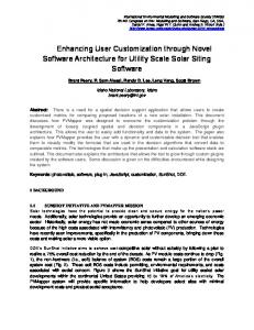
Figure 1: Overview. Frame field design over surfaces is typically guided by constraints on (an)isotropy, lengths, and feature alignments (left). While current methods (e.g., MIQ [Bommes et al. 2009]) use the Euclidean-induced metric to find an appropriate frame (and further derive a quadrangulation, top), our method (bottom) first customizes a Riemannian metric from the design requirements, then generates a frame field that is a smooth cross field in this new metric—thus offering a more flexible and more intuitive design process producing high quality frame fields. Metrics are visualized using their local unit circles (middle left); the resulting frame’s sizes and directions are indicated as color isocurves (middle right); and a quadrangulation based on the frame field is then automatically extracted (right).

Abstract

1

This paper presents a new technique for frame field generation. As generic frame fields (with arbitrary anisotropy, orientation, and sizing) can be regarded as cross fields in a specific Riemannian metric, we tackle frame field design by first computing a discrete metric on the input surface that is compatible with a sparse or dense set of input constraints. The final frame field is then found by computing an optimal cross field in this customized metric. We propose frame field design constraints on alignment, size, and skewness at arbitrary locations on the mesh as well as along feature curves, offering much improved flexibility over previous approaches. We demonstrate the advantages of our frame field generation through the automatic quadrangulation of man-made and organic shapes with controllable anisotropy, robust handling of narrow surface strips, and precise feature alignment. We also extend our technique to the design of n-vector fields.

Frame fields on discrete 2-manifolds are key to a wide range of applications in computer graphics, including texture mapping and quadrangulation remeshing, as they induce a smoothly-varying assignment of a basis for all the tangent spaces of the surface. While orthonormal frame fields (also called 4-symmetry direction fields or cross fields) are most common due to the convenience afforded by unit and orthogonal bases, the need for non-uniform, anisotropic, and skewed frame fields has grown tremendously in recent years due to their versatility in geometry processing.

CR Categories: I.3.3 [Computer Graphics]: Computational Geometry & Object Modeling—Curve & surface representations. Keywords: Frame field generation, metric customization, n-vector field design, geometry processing. ∗ Corresponding

authors: [email protected], [email protected]

Introduction

However, the design of generic frame fields remains a challenging task: one has to balance user-input or application-driven requirements (such as alignment to given directions and sizing constraints) with the resulting smoothness of the frame field and its inevitable singularities. Depending on the targeted application, input constraints can be either under- or over-constrained, as smoothness and direction constraints may conflict and interfere with sizing constraints, and vice-versa. This renders any user-guided design process long and tedious: automatic frame field generation can result in inaccurate alignments, requiring constraints to be interactively added or removed until the final frame field is acceptable. In this paper, we argue that frame field design is best accomplished by first designing a non-Euclidean metric on the surface based on the input constraints, and then deriving the frame field as an orthonormal frame field in this computed metric. Abandoning the viewpoint that the surface is embedded in Euclidean space and considering instead the more general case of Riemannian manifolds significantly increases flexibility in the design of frame field, resulting in a tighter control over directional and sizing constraints.

1.1

Related work

We first review the key previous works that we will build upon or extend in our metric-based approach to frame field generation.

Orthonormal frames. Initially proposed by Hertzmann and Zorin [2000] for cross-hatching rendering, cross field design has been extensively studied ever since [Palacios and Zhang 2007], whether through connections derived from the specification of the cross field singularities [Ray et al. 2008; Crane et al. 2010], or through a smooth interpolation of a sparse set of directional constraints [Ray et al. 2009; Bommes et al. 2009; Kn¨oppel et al. 2013]. However, cross fields do not encode local scale or anisotropy, which is a severe limitation in the context of meshing where control over sizing and shape of elements is paramount. Arbitrary frames. Cross fields were quickly extended to more general frame fields. Liu et al. [2011] first proposed to use conjugate direction fields to handle frames with nonorthogonal vectors, but failed to offer control over the lengths of basis vectors. Diamanti et al. [2014] generalized n-symmetry fields to n-vector fields by removing the rotation symmetry assumption, while Panozzo et al. [2014] introduced a more general frame field construction by composing a stretching field and a cross field. However, when used for parameterization or quadrangulation, their approach involves the embedding in 3D Euclidean space of a deformation of the mesh. This intermediary step imposes strong restrictions on the resulting frame field, as only fields that can be warped into a cross field by deforming the input mesh in R3 can be obtained. The design space of frame fields is thus unnecessarily restricted, since traditional applications of frame field design such as quadrangulation do not require (or even benefit from) such constraints. Metric optimization. Metric tensor fields have received increasing attention in computer graphics [de Goes et al. 2014], in particular for remeshing [Ling et al. 2014]. A first series of works looked to equip a surface with a flat metric with singularities [Jin et al. 2007; Ben-Chen et al. 2008]. Metrics that are conformal to the original surface metric induced by R3 were also targeted [Jin et al. 2004; Springborn et al. 2008; Myles and Zorin 2012], but offered very limited user control. More recently, the interplay between metrics and frame fields was leveraged to derive low-distortion parameterization with alignment constraints [Myles and Zorin 2013] and adaptive remeshing [Lai et al. 2010] through the computation of a flat cone metric. Methods generating frame fields through harmonic interpolation of symmetric matrices [Panozzo et al. 2014] or polynomial coefficients [Diamanti et al. 2014] can also be regarded as ways to approximate metrics satisfying user-specified constraints through linear systems. These metrics are then further improved through additional deformation steps for practical applications such as global parameterization. Our work extends this line of work by directly constructing a customized metric to offer much increased flexibility and user control in the frame field design. Additionally, our logarithm-based formulation can handle rapid scale changes in the metric, further improving upon the approach of [Panozzo et al. 2014] whose deformation step already produced fewer additional singularity than [Diamanti et al. 2014].

1.2

Contributions

In this paper, we approach the design of an arbitrary frame field through the construction of an orthonormal frame field in a customized metric. From input constraints on direction, size, and angle for the frame field, we first construct a Riemannian metric g, discretized as a 2×2 matrix on each mesh triangle, which accounts for angles and sizing constraints. Once the Riemannian metric has been computed, robust state-of-the-art tools can be directly leveraged to derive the final frame field since it amounts to finding a simple cross field in this metric g; that is, the desired frame field is g-orthonormal by construction of the metric. We demonstrate through a variety of examples that the frame fields designed through our approach are

significantly more general than previous methods; in particular, fine control over anisotropy and precise feature curve alignment can be simultaneously enforced, unlike in previous approaches. We also show the versatility of our method by extending it to n-vector fields.

2

Frame Field Design Principles

When designing a frame field, one needs to set constraints on direction, size, angle, and combinations thereof. These (often sparse) constraints will then guide the creation of the field by enforcing that it tightly aligns to application-dependent or geometrically-relevant directions, forms preset angles to accommodate acute corners, or varies in size to better adapt to local features. Generating a frame field from these constraints therefore requires to determine a wellbehaved (i.e., piecewise smooth and visually least-varying) frame field fitting the constraints. As we mentioned early on, one of the challenges for the user or any automatic application-specific assignment of constraints is to define requirements that are not conflicting with each other, so that the impact of each constraint on the resulting frame field is intuitive. We thus need to provide simple, atomic primitives that one can automatically or manually input to guide the generation of the desired frame field.

2.1

Design primitives

Whether it be for a user designing the properties of a parameterization or for an automated creation of guiding fields to quadrangulate a surface, we assume there are only two types of key primitives: ● Local primitives: automatic or user-specified requirements can be formulated at various locations on the surface. One should be able to indicate both the direction, and potentially the magnitude, of one or two of the basis vectors of the frame. Similarly, the frame field could be required to be isotropic (i.e., a scaled Euclidean orthonormal frame) at some key places over the surface. ● Curve primitives: design requirements should also accommodate the specific layout of the frame field tangentially to 1D curves such as boundary curves, sharp features, and user-sketched curves with controllable skewness and sizing adaptation to, typically, local geodesic curvatures. These two basic sets of design primitives will be implemented in our approach as a series of constraints on (a subset of) triangles. That is, while the interface (to the user, or to our frame field generator) offers the set of primitives described above, our algorithm manipulates their associated constraints instead in order to generate a frame field as we now detail.

2.2

Frame constraints

We formulate the mathematical constraints corresponding to our design primitives on a per-triangle basis as we will generate a frame field F over an input triangulated surface by assigning a frame Ft per triangle t. Our constraints are separated into two families, one containing alignment requirements A to either local directions or (feature/user-specified) curves, and one handling sizing requirements S. Each family includes a list of associated constraints on selected triangles—either isolated triangles if they come from a local design primitive, or strips of triangles adjacent to a (feature, boundary, or user-drawn) curve if they are generated from curve primitives. We will use d and n to represent directions, i.e., vectors that are unit in the original Euclidean-induced metric g¯. The sizing constraints set is composed of the union Ss ∪ Sd ≡ S of two different types of frame requirements: – Uniform scaling requirement (Ss ): for (t, s) ∈ Ss , the magnitude of the g-orthogonal frame Ft ’s two basis vectors must be s ∈ R+ on triangle t;

– Directional length requirement (Sd ): for (t, d, l) ∈ Sd , one basis vector of the frame Ft must be along the direction d with a magnitude l ∈ R+ on triangle t. The alignment constraints set is denoted as A ≡ Ad ∪Ac , and contains requirements of two types as well: – Directional alignment requirement (Ad ): a directional alignment requirement (t, d) ∈ Ad asks for a basis vector of the frame Ft in triangle t to be aligned with a given direction d; – Curve alignment requirement (Ac ): a curve alignment requirement (t, d, n, r) ∈ Ac uses a unit tangent d to a (feature or userdrawn) curve and another (typically normal) direction n pointing away from the curve. Ft is then asked to be aligned with d, while the rate of change along n of the magnitude of the basis vector aligned with d must be r ∈ R. Effect of requirements. The user can then define one or several of these constraints per triangle of the input mesh in order to guide the frame field to her taste. All these constraints have rather intuitive geometric interpretations. The first sizing constraint asks for the local frame to be a rescaled version of the unit orthonormal frame; this type of constraint will control the local scale s of the frame field, which will therefore enforce local conformality of a quadrangulation built from the frame field. The second type of sizing requirements allows the user to set both the direction and magnitude of one of the basis vectors of the frame F , offering directionality and sizing control of the frame on a triangle of the surface mesh. Similarly, the alignment constraints will eiAc ther force the frame field to be aligned with a given unit direction d, or, if two such constraints are set for the same triangle, the Ad Sd frame on this triangle will be entirely defined via these two (different) directions, thus alSs lowing easy control of local skewness. The last constraint is of a different nature: it brings a direct control of alignment along a curve and a differential control of length away from the curve. That is, it requests that one of the basis vectors of a frame be aligned with a curve and that it stretches/shrinks in size at a certain rate along a given “normal” direction (see inset), while remaining of a similar size along the tangential direction. This type of constraints provide users with a very convenient way to control not directly the size of a frame’s basis vector along a user-sketched curve or feature, but its differential behavior. We will show (see App. B) that in fact, if the rate of change r is set to be the geodesic curvature of the curve, the resulting frame field will perfectly adapt to the curve both in terms of direction and relative size (see Fig. 5). Setting an arbitrary rate r and an arbitrary direction n allows more flexibility to adapt, for instance, to geometry and additional attributes. Additional requirements. Notice that unless the user purposely defines several conflicting directional constraints in a same triangle our frame constraints are never in conflict, by construction. We will show in the remainder of this paper that the requirements above are flexible enough for a user or artist to guide the generation of frame fields. We can, in fact, add more involved constraints which have much less obvious geometric interpretations since they involve constraints that are not directly imposed on the basis vectors of the frame—but on arbitrary directional derivatives of the metric induced by the field. We will limit our exposition to the simple constraints listed above, as it will be fairly straightforward to infer these possible additional requirements from our numerical treatment of the design process.

2.3

Computing an optimal frame field – a first glance

Once a list of constraints A ∪ S has been input, we proceed in two steps. First, we compute a metric g that satisfies all the metricdependent requirements as described in Sec. 3, before generating the frame field as a smooth g-orthonormal frame field that best satisfies the direction-dependent requirements as described in Sec. 4. What constitutes a metric-dependent constraint vs. a direction-dependent constraint is left hidden to the user, since the creation of a discrete Riemannian metric is only used as a means to an end. However, we will demonstrate that this detour via a metric not only grows the space of possible frame fields, but also allows us to use robust, existing methods that facilitate the implementation of our approach and help enforce the constraints. Discrete metrics. We will assume that a surface is provided in the form of a simplicial complex M in R3 . Each triangle t of the mesh ¯t (for instance, aligned is arbitrarily assigned an orthonormal basis B to one of its edges). The metric of the surface induced by the Euclidean space is denoted g¯, and encoded per triangle as the identity ¯t . Recall that, to improve legibility, we matrix Id in each frame B will denote directions by d or n (i.e., vectors that are unit in metric g¯); general vectors (of arbitrary magnitude) will be denoted u or v instead. Finally, we encode an arbitrary Riemannian metric g by storing it as a symmetric positive-definite matrix gt per triangle ¯t for simplicity. using the same reference coordinate frame B Discrete connections. For the metric g¯, the union of two adjacent triangles t1 and t2 is intrinsically flat since one can use the “hinge map” to flatten the pair into R2 without inducing any intrinsic dis¯ t1 t2 that rotortion. Consequently, there exists a rotation matrix R ¯t1 by an angle of θ¯t1 t2 to the adjacent tates the coordinate system B ¯t2 in this flatten configuration (and obviously, coordinate system B ¯ tT t is simply the inverse rotation) [Ray et al. 2009]. This ¯ t2 t1 = R R 1 2 ¯ for g¯ as rotation represents a canonical (Levi-Civita) connection ∇ it enables us to measure the difference between vectors living in adjacent triangles by parallel-transporting them into the same tangent space before comparing them [Crane et al. 2010]: a vector ut1 stored ¯t1 can be parallel transported in the original metric g¯ of in basis B ¯ t2 t1 ut1 in t2 , this time expressed the surface as the vector ut2 = R ¯ in basis Bt2 . Note that the idea of parallel transport extends to an arbitrary metric g—but the expression of the associated Levi-Civita connection Rt1 t2 is more involved as g is unlikely, in general, to be flat in the union of two adjacent triangles. We will, however, provide a closed-form approximation for this rotation matrix in Sec. 4. Metric smoothness. With this parallel transport, we can now measure how much a metric g locally changes (with respect to the reference metric g¯) between adjacent tangent spaces as well: if two vectors ut1 and vt1 live in t1 , their inner product in gt1 is uT t1 gt1 vt1 , while the inner product of these same vectors paralleltransported to t2 become uT t2 gt2 vt2 in gt2 . As a consequence, the difference of metric between two adjacent triangles t1 and t2 is ¯t1 as: gt1 − R ¯ tT t gt2 R ¯ t2 t1 (or similarly in B ¯t2 as: expressed in B 2 1 T ¯ ¯ Rt1 t2 gt1 Rt1 t2 − gt2 ). This difference corresponds to the integral ¯ of the continuous notion of the g¯-induced covariant derivative ∇g ¯g = 0 as exalong the dual edge between t1 and t2 . (Notice that ∇¯ pected since we use the metric g¯ as a reference.) The matrix norm of this difference (here, the Frobenius norm since we express 2-tensors as matrices in orthonormal bases) is thus a scalar measure of how the metric locally changes. From metric to frames. Finally, note that if an arbitrary discrete metric g is defined via its matrix per triangle, then it is a trivial matter to derive a g-orthonormal basis B (i.e., a frame field that is both orthogonal and unit when measured in the metric g) from our refer¯ through: B = B( ¯ √g)−1 – i.e., the basis vectors of B ¯ ence basis B

Uniform scaling. If a uniform scaling requirement (t, s) ∈ Ss is set on triangle t, the metric g must be locally conformal to the original metric g¯ with a conformal factor s2 , i.e.,

1 Id . (2) s2 This type of constraints is useful in the context of quadrangulation for regions where square-shaped elements are desirable (see Fig. 2). gt =

Figure 2: Sparse constraints. A sparse set of uniform scaling constraints (color facets, left) or angle constraints at feature curve intersections (right) is enough to create smooth frame fields. are easily deformed into the basis vectors of B knowing g, where B ¯ as columns of matrix stores its two basis vectors (expressed in B) Bt for each triangle t. Note that this basis Bt is not locally coher¯ itself was randomly chosen to ent on nearby triangles, as the field B start with. However, a g-orthonormal frame field F that closely fits specified frame requirements can then be computed from frame B as a simple rotation angle per triangle, turning B into F : this pure rotation in metric g of each frame Bt preserves the g-orthonormality of the resulting frames, but will allow us to enforce smoothness and frame constraints. Finally, note that the actual frame field F will not ¯ depend on the choice of B—this latter basis is only used to encode the vector basis of F .

3

Metric Customization

A Riemannian metric on a 2-manifold is a symmetric positivedefinite tensor field g that defines the inner product of two tangent T vectors u1 and u2 through uT 1 gu2 , with u gu > 0 for any nonzero vector u. In this section, we present how a subset of the user constraints are used to generate such a Riemannian metric g on the input triangle mesh. The role of this discrete metric will be to turn the generation of an arbitrary frame field into the much simpler and well-studied case of finding a cross field, where orthogonality and unit norm are defined by this customized metric g.

3.1

Directional length constraint. Metric g can also be constrained in terms of its notion of length in given directions. – Single constraint. If a triangle t has only one directional length constraint (t, d, l) ∈ Sd , the fact that F must be unit in g implies:

1 . (3) l2 This directional length constraint can directly be used to ensure that the size of elements along feature curves are well adapted, to avoid large approximation errors. One can follow the method of [Alliez et al. 2003], where a local size l is determined by a Hausdorff-based error tolerance ε and the geodesic curvature κ of the feature to automatically set constraints along the feature curve: we simply use directional length constraints on triangles adjacent to the feature curve using its tangential directions d, with their lengths l set to: √ l = 2 ε(2/∣κ∣ − ε). (4) dT gt d =

We set ε to be 10−4 times the bounding-box diagonal span in all our results. This adaptation of length and direction (possibly after clamping of the length l to a user-specified range [smin , smax ] for robustness) provides a fine sizing control of the frame field near sharp features as demonstrated in Fig. 3. – Double constraint. When two directional length constraints (t, d1 , l1 ), (t, d2 , l2 ) ∈ Sd are present on the same triangle t, the local frame is entirely fixed as Ft = (l1 d1 , l2 d2 ). Since F must be g-orthonormal, we must impose that the metric g satisfies: dT 1 gd1 =

Metric constraints

As discussed above, a metric defines the inner product of tangent vectors. It thus determines lengths and angles of vectors. Consequently, any frame field requirement involving length or angles does also define, implicitly, local constraints on the metric. From the frame constraints given in Sec. 2.2, we extract all the implicit metric constraints such that the frame field requirements correspond, in a (currently unknown) metric g, to a smooth, unit and orthogonal frame field: once these metric constraints are identified, we will simply find the metric g as a matrix field stored in the canonical ¯ through optimization in order to best fit the metric frame field B constraints. In fact, aside from requirements that involve a single directional alignment constraint (and thus, for which the metric g is unconstrained), all of our frame requirements impose some form of metric constraints per triangle as we now go over.

1 , l12

dT 2 gd2 =

1 , l22

and

dT 1 gd2 = 0.

(5)

Note that this double constraint is particularly convenient to adapt a frame field to the principal curvature directions of a surface and its curvatures: evaluation of the shape operator and its principal curvature directions on each input triangle provides such constraints, see Figs. 4, 9, and 13. Geodesic curvature. If (t, d, n, r) ∈ Ac , the magnitude of d in the metric g must be stretching along direction n at a rate r. (Note that we purposely restricted this constraint to use a direction (i.e., g¯-unit) vector n for simplicity; an arbitrary vector u could be used instead, as one just has to rescale r by the norm of u to enforce this generalized constraint.) Using the directional derivative in the orig¯ to conveniently re-express this constraint, this means inal metric ∇

Angle constraint. If two directional (alignment or length) constraints (t, d1 ⋯), (t, d2 ⋯) ∈ Ad ∪ Sd are set on the same triangle, the two (¯ g -unit) directions d1 and d2 on t fully determine the directions of frame Ft . Since F must be an orthogonal frame field with respect to our customized metric g, the metric at t should satisfy

dT 1 gt d2 = 0.

(1)

Such angle constraints are particularly convenient to fix frame field directions at corners, see Fig. 2.

Figure 3: Sizing control of boundaries. Sizing is easily controlled (left), even along complex boundaries as demonstrated by the resulting frame-driven quadrangulation (right).

(since a rate change r implies an exponential-of-r growth) that one must enforce: 1 ¯ n (ln(dT gd)) = r. ∇ (6) 2 In fact, this metric constraint has a very simple geometric interpretation (see Fig. 5): if n is the normal to the feature (i.e., nTg¯d = 0) and r is the local geodesic curvature κ of the feature curve we are trying to adapt to, then this constraint reflects the fact that the (feature or user-drawn) curve must be a geodesic in the metric g (see proof in App. B). Hence, its general form where n and r are arbitrarily chosen imposes a geodesic curvature condition on g. Imposing a feature alignment constraint on the triangles at the boundary of a simple disk for instance (inset) forces proper alignment and curvature-adapted sizing of the quads there, pushing the singularities deeper inside.

λ∗ = 1

Figure 5: Metric smoothness control. For geodesic curvature constraints along features (ωc = 0.6), reducing λ∗ enhances frame smoothness at the price of more rapidly changing quad sizes. ¯ 2 ln g is the biharmonic energy of ln g. The relative weight term ∇ λ thus offers the typical tuning between what amounts to a membrane and a thin shell energy on the metric: smaller values of λ will result in wider frame size ranges, with also more singularities to accommodate the rapidly changing size; larger values of λ will create smoother variations of the resulting metric, see Fig. 5. Metric discontinuity across features. In order to allow flexible (and sparse) control over anisotropy, it is important to relax the smoothness requirement across feature curves. This is easily achieved by simply considering features as boundaries: neither the covariant derivative nor the Laplacian are used on dual edges crossing a feature. Note that the metric and the resulting frame field will still have the desired continuity for two reasons: first, the length along the tangential direction across the normal direction will be forced to be continuous due to our differential constraint (Eq. 6); second, alignment to the feature direction will force the nearby frames to align to both the tangential and normal directions.

3.3 Figure 4: Feature and curvature alignments. Requiring feature alignments (red curves), local alignment to principal directions, and sizing constraints (blue regions) on the aircraft model (left) results in a frame field (right) generating a high-quality quad mesh (middle).

3.2

Metric customization through optimization

With all the relevant frame requirements converted to their implied metric constraints, we must now find the best metric field g, defined ¯t ) per triangle of as one matrix gt (stored in the predefined frame B the form: g g12 gt = ( 11 ). g21 g22

λ∗ = 0.6

Numerical formulation

We rewrite the previous constrained energy as an unconstrained minimization in the log of g, where each type of constraint is enforced via a penalty energy. In order to maintain consistency in the units of the energies, we enforce the non-logarithm-based metric constraints (appearing in Eqs. 1, 3, and 5) of the type dT 1 exp(g)d2 = c, c ≥ 0,

(7)

using a penalty P expressed as: P (d1 , d2 , c, g) = ln ∣d1 +d2 ∣2eg −ln(∣d1 ∣2eg +∣d2 ∣2eg +2c),

Since each gt must be symmetric positive-definite (SPD) for the field to define a proper Reimannian metric, we must also constrain 2 g21 = g12 , det g = g11 g22 − g12 > 0 and tr(g) = g11 + g22 > 0. The need for inequality constraints can be removed if one parameterizes the space of SPD matrices gt through the space of symmetric matrices gt with gt = ln gt , where ln is the matrix logarithm. Indeed, for any symmetric matrix g, the matrix exponential gt = exp(g) is SPD. Consequently, we can formulate without inequalities the customization of the metric g as a constrained optimization: we ask for the smoothest metric that fits the input constraints through argmin ∫ g

¯ ln g∥2 + (1 − λ)∥∇ ¯ 2 ln g∥2 ds λ∥∇

M

subject to all metric constraints, ¯ and its associated where we use both the covariant derivative ∇ ¯ 2 defined in the metric g¯ (see Sec. 2.3) to meaLaplacian operator ∇ sure a Sobolev-like smoothness of the log of the metric field. Besides being the canonical differential operators on the input surface, note that when g is conformal, the first term in this measure reduces to the usual Dirichlet energy of the conformal scaling. The second

Figure 6: Metric customization. Using double constraints per triangle based on local principal curvatures, our metric optimization (right) drastically decreases the alignment error ∥F −Tg −1F −1 −I∥2 compared to the original surface metric g¯ (left). Metric g is visualized through its local unit circles.

where ∣u∣2eg = uT exp(g)u , and the cosine law was used to ensure that the logarithm is only applied to positive values. To decrease non-linearity, all double constraints F = (l1 d1 , l2 d2 ) can be directly expressed in matrix form as: (l1 d1 , l2 d2 )T exp(g)(l1 d1 , l2 d2 ) = Id, and recast into a simple linear constraint in log space as: g = ln(F −T F −1 ), −T

−1

where ln(F F ) is easily computed as the diagonal matrix formed by the logarithm of eigenvalues in the eigenbasis of F −T F −1 . We can now numerically solve for the optimal metric field g through the following minimization: 1 ws wd wc argming Es + ES + ES ∪A + EAc ∣M∣ ∣Ss ∣ s ∣Sd ∪ Ad ∣ d d ∣Ac ∣ ∣ti ∣+∣tj ∣ ωc ∗ ⎧ ⎪ ¯ tT t gt R ¯ t t ∥2 ⎪ Es = (1 − )λ ∑ ∥gti − R ⎪ j j i j i ⎪ 100 2 ⎪ ⎪ (ti ,tj)∈N ⎪ ⎪ ⎪ ⎪ ⎪ ωc ∗ ⎪ ¯ tT t gt R ¯ t t )∥2 ⎪ + (1 − (1 − )λ ) ∑ ∣t∣ ∥ ∑ (gt − R ⎪ i i i ⎪ ⎪ 100 ⎪ t∈M ti ∈Nt ⎪ ⎪ ⎪ ⎪ ⎪ 1 2 ⎪ ⎪ ⎪ ⎪ ⎪ ESs = ∑ ∣t∣ [gt − ln( s2 Id)] with ⎨ (t,s)∈Ss ⎪ 2 ⎪ ⎪ ⎪ E ∣t∣ [P (d1 , d2 , c, gt )] ∑ S ∪A ⎪ d d = ⎪ ⎪ ⎪ (t,d ⋯),(t,d ⋯)∈S ∪A 1 2 ⎪ d d ⎪ ⎪ ⎪ ⎪ ¯ n ln ∣d∣2exp(gt ) −2r]2 ⎪ [ ∣t∣ ∇ E = ∑ A ⎪ c ⎪ ⎪ ⎪ (t,d,n,r)∈Ac ⎪ ⎪ ⎪ ⎪ ⎪ ⎪ ∣t∣+∣t 2 n∣ ⎪ ⎪ [ln ∣d∣2exp(gt ) − ln ∣d∣2R¯ T exp(gt )R¯ t t ] , ⎪ ⎩ + n n tn t 2 where N denotes the pairs of adjacent triangles that are not across a feature, Nt is the set of adjacent triangles to t that are not across a feature (i.e., usually three triangles, except near a feature to allow for rapid sizing change), and tn denotes the triangle pointed by n from ¯ t so that we can enforce Eq. 6 properly with EAc . The ∇-based smoothness energy Es , combining both the covariant derivative and the Laplacian of the logarithm of g, forces the metric g to be smooth everywhere except across feature curves by construction. This energy is then added to an area-weighted sum of penalty terms on any unfulfilled metric constraints, where we used ∣t∣ to denote the area of triangle t, ∣M∣ for the total surface area of the input mesh, and by extension, we used ∣S∣ for any constraint set S to denote the total area of the triangles included in S. This area weighting, along with the consistent use of log-based constraints, renders the tuning of the three parameters independent of the model and very intuitive: the weights on each type of constraints can be adjusted to give some constraints precedence over others. Finally, note that we selected the tuning parameter λ of the smoothing energy Es to depend both on a smoothness coefficient λ∗ and the geodesic curvature enforcement weight ωc : by choosing λ = (1 − ωc /100)λ∗ , we make sure that the impact of the geodesic curvature constraint is not too weakened by a large smoothness coefficient. We use λ∗ = 0.95, ws = wd = wc = 0.01 in all our examples to balance metric smoothness and constraint enforcement; exceptions to these default parameters will be clearly marked in their associated caption—see for instance Fig. 5, where we demonstrate the effect of λ∗ to the results. Note that, since Es and ESs are quadratic terms, the non-linearity of this energy boils down to the computation of the matrix exponential of exp(g). Because the matrices gt are symmetric and real, their exponentials can be computed in closed form, avoiding the well-known complexity of matrix exponentiation [Moler and Loan 2003]. We use Maxima [Schelter 2015] to automatically derive the gradient and

Hessian of the closed form exponentiation. The resulting energy being non-convex and highly nonlinear, we use a Sequential Quadratic solver to optimize it starting from an identity metric (the original Euclidean induced metric g¯) as the initial guess. As we demonstrate in Sec. 5, this unconstrained minimization converges quickly to a solution that fulfills the metric constraints remarkably well. The Pegasus example in Fig. 6 demonstrates that, while the original metric g¯ generates metric constraint errors in the range [700, 105 ], the optimized metric g quickly converges to errors in the range [0.02, 22], with 90% of the triangles having errors below 4.

4

Frame Field Generation

A frame field can always be regarded as a locally stretched cross field, as exploited in [Panozzo et al. 2014] which pulls back a cross field from a deformation of the original surface. In our approach, we generalize this idea by, instead, considering that frame fields are cross fields in some Riemannian metric g. Since we customized a metric g to be compatible with our frame requirements, all we need to obtain a desirable frame field F now is finding a smooth cross field in this metric that accounts for the remaining alignment (nonmetric) constraints.

4.1

Orthonormal basis for metric g

¯ was arbitrarily chosen by picking a set of Recall that the basis B ¯t per triangle t. Now that we have equipped g¯-orthonormal frames B our surface with a discrete Riemannian metric g, we can trivially derive a g-orthonormal basis B through the following procedure. For each SPD matrix gt in triangle t, we compute the√(symmetric positive-definite) principal square root matrix Gt = gt whose eigenvalues (representing principal stretches) are the square roots of the eigenvalues of g associated with the same eigenvectors. Then, the basis B defined such that: ¯t G−1 Bt = B t

∀t ∈ M

¯ ¯-orthonormal. Note is g-orthonormal since gt = Gt GT t and B is g that this is not our frame field yet: this is merely a canonical set of coordinate systems on triangles adapted to the metric g.

Figure 7: Frame field gallery. Using principal curvatures and their directions, along with minimal user interaction if desired, smooth geometry-adapted frame fields are simple to generate.

4.2

Connection of metric g

In order to find the final frame field F , we need to define a proper way to measure the spatial variations of a vector or frame field in the metric g so that we can find the smoothest g-orthonormal frame fitting the constraints. The role of the Levi-Civita connection in a given metric has been proposed in a variety of works for exactly this purpose of smoothness measurement, e.g., [Bommes et al. 2009; Ray et al. 2009; Crane et al. 2010]. We adopt the same approach here, and rely on the discrete connection R, defined as a rotation Rti tj between pair of adjacent triangles ti and tj , which is LeviCivita (torsion-free) in the metric g. However, this connection is ¯ g is no longer less easy to compute than the canonical connection R: locally flat in general. Fortunately, the continuous expression of the Levi-Civita connection in a metric g is well known: if one uses a local parameterization ¯ = (∂/∂u, ∂/∂v), the angle θ by (u, v) based on a local basis B which a tangent vector rotates along a finite path γ when parallel transported by the Levi-Civita connection of g is [Oprea 2007]: θ = ∫ (G11,v −G21,u , G12,v −G22,u ) γ

G du ( ), det(G) dv

(8)

where G is the principal square root of g, Gpq represents its p-th row and q-th column element of G in the (u, v) coordinates, and Gpq,u (resp., Gpq,v ) represents the spatial derivative of this element along u (resp., v). See App. A for a short derivation of this fact. We can thus approximate the rotation Rti tj based on our discrete version of the metric g, as the angle θij along dual paths between adjacent triangles for each pair of triangle ti and tj . Since our discretization only has a piecewise constant field G, we first evaluate an average Gij per edge midpoint by computing the average gij of ¯i as: g in the local frame B 1 ¯ tT t gt R ¯ t t ). (gt + R j j i j i 2 i √ We deduce Gij through: Gij = gij . With a matrix G evaluated at the midpoints of the three edges, we simply linearly interpolate G in the (u, v) coordinate system to get the required first derivatives involved in the integral in Eq. 8 along the half dual edge, which can then be evaluated in closed form. (Note that this piecewise linear interpolation amounts to using Crouzeix-Raviart non-conforming basis elements for the edge values of G.) By summing the angles of two consecutive half dual edges and θ¯ij , we immediately deduce the angle θij —which, consequently, results in a rotation matrix Rti tj by this angle, thus providing a concrete approximation of the LeviCivita connection of g. Note that adding θ¯ij is necessary to align ¯i G−1 ¯ −1 B ij and Bj Gji . This averaging procedure followed by linear interpolation was chosen so that Eq. 8 can be performed analytically; other more involved interpolation of G or g can be used instead, but our simple approximation resulted in similar angles in all our tests. See App. A for how to evaluate Rti tj in practice.

B and alignment constraints. In our implementation, we adopt the popular 4-symmetry direction field representation used in [Palacios and Zhang 2007], where a representative vector ut per triangle t expressed in basis Bt is found such that the resulting vector field u minimizes the following non-linear energy: argmin

∥uti − Rti tj utj ∥2 (4)

∑ ti ,tj adjacent

+ wa

∑

∥ut −Gt d(4) /∣Gt d∣ ∥2

(t,d⋯)∈Ad ∪Sd 2 + wu ∑ ∥uT t ut −1∥ , t∈M

where the superscript ⋅(4) is used to indicate that one must quadruple the angles of the connection R, and that each direction d in triangle t must also be expressed in B (through Gt d) before having its resulting angle with the first basis vector of B being quadrupled to ensure a 4-RoSy. Note that the last term enforces the vectors ut to be unit (in metric g, since vectors are expressed in the bases Bt ), the first term ensures smoothness with respect to the (quadrupled) connection R, while the coefficient wa allows the user to control how much to favor direction alignments over sizing, as shown in Fig. 8. Once u is computed, the angle αt per triangle t is found by dividing the angle that ut makes with the first basis vector in B by 4. The resulting frame field F will thus be computed as, for each triangle t, the frame Bt rotated within t by αt . By construction, this optimized frame field is smooth and with the required sizing as shown in Fig. 7.

gij =

4.3

Cross Field Generation

Once the basis B and connection R associated with our customdesigned metric g are known, the final frame field generation amounts to computing a cross field in B that is smooth with respect to the connection R. Recall that the frame requirements contain a series of direction alignment constraints per selected triangle; we thus need a rotation angle αt of the frame Bt for each triangle t so that the resulting frame F closely satisfies these alignment requirements, while being optimally smooth in the Levi-Civita connection of g. Finding such a cross field is well studied, and a number of robust methods exist for which one simply needs to provide the connection

Figure 8: Size vs. alignment. With constraints on feature curves (red), directions (blue arrows) and uniform scaling (0.1 in blue, 0.6 in red), frame fields are generated with λ∗ = 0.5, ωc = 3; we use wa = 1×10−5 (left) or wa = 3 × 10−3 (right). Larger wa lead to better direction alignment, but control over scaling worsens.

5

Applications and Results

Frame fields have a multitude of applications in computer graphics. In particular, we demonstrate the utility of our frame field design in quadrangulation. We also present a straightforward generalization of our approach to n-vector field design.

5.1

Quadrangulation

Once a frame field has been generated, several state-of-the-art tools (e.g. [Panozzo et al. 2014]) can be employed to derive quadrilateral meshes. We implemented our own frame-driven quadrangulation technique to produce results with similar quality and improved efficiency by computing cross-field guided parameterization. Denoting the parameterization as the function f = (f 1 , f 2 )T ∶ M → R2 , we seek to align the isocurve directions of f to the basis vectors of the frame field F , and match the spacing between isocurves to the magnitude of the basis vectors. This requirement is met if the Jacobian df = (df 1 , df 2 )T of f is dual to F, that is, if df i (Fj ) = δji , where δ is the Kronecker delta. Thus, we find our parameterization by opti-

Figure 9: Meshing. With only double constraints derived from the curvature tensor, the resulting quad meshes automatically adapt to the geometry of the input model. mizing the following target function: ∥df F − I∥2 dA.

argmin ∫ f

(9)

M

A transition function is introduced based on the given frame field as recommended in [Bommes et al. 2009] to create a seamless parameterization across regions where different choices of alignment of df 1 to the 4 vectors in the g-orthonormal 4-vector field exist. From the resulting parameterization, the libQEx tool [Ebke et al. 2013] is able to robustly generate the final quad meshes without postprocessing. Results. We demonstrate the versatility and robustness of our approach through a series of results on meshes including sharp features, narrow strips of surfaces, and acute angles. First, we show results where no user interaction has been used: using only automatic evaluations of the curvature tensor to impose double constraints along principal curvature directions, we already obtain high quality quad meshes on complex models, e.g., in Figs. 9 and 13.

Fig. 10 offers a comparison of our approach with current frame field methods. On this model without sharp features, our approach leads to slightly improved results (straighter elements) compared to [Panozzo et al. 2014], due to our more general connection and log space on this example of rapidly changing scale; the approach of Diamanti et al. [2014], instead, fail to adapt simultaneously to both size and direction constraints as it relies on the Euclidean-induced Levi-Civita connection only. When sharp features are present, existing methods such as [Panozzo et al. 2014] fail to offer control over anisotropy even on basic models as shown in Fig. 11. Our differential metric constraints allowing for normal discontinuity of the metric leads to an intuitive and flexible design of the frame field: the metric continuity along the feature curves can be enforced without restricting the anisotropy across the feature curve. Thus, with a sparse set of anisotropic length constraints, we automatically find a solution that ensures quad edges along features to match up, while the edges orthogonal to features can have drastically different lengths to accommodate different anisotropic constraints on the two sides of each feature. Our method can also directly handle CAD models with numerous sharp features and narrow parts. For instance, the beetle model contains narrow strips between the windows (Fig. 1) and the Sydney model in Fig. 12 has complex directional size constraint along ridges; yet we can layout good quad meshes for both examples. The flexibility offered by our metric also leads to a high quality quad mesh for CAD models with acute angles formed by the intersections of sharp features (Fig. 15), which usually present an extreme challenge for traditional quadrangulation methods. The statistics on all our models are given in Tab. 1. Timing was measured on a computer with an Intel Core i7-2600k processor and

(a)

(b)

(c)

(d)

Figure 10: Comparisons. With the same rapid change of size constraints, our method ((a),(c)) produce straighter quads near the front than [Panozzo et al. 2014] (b). Compared to [Diamanti et al. 2014] (d), our result demonstrates much improved singularity distribution. 16GB memory. The average relative size deviations and average angle deviations provide a measure of how well the input constraints are satisfied; they do not necessarily provide a good measure of quad mesh quality. Note that computation times do not depend only on model size, but also on the non-linearity of the constraints. More direction size constraints induce more non-linearity, thus making the problem harder to solve. Also, for the two Sculpture models, adding the Laplacian smoothing term makes the Hessian matrix denser, hence increasing processing time. Models

#T

Sculpture-1 Sculpture-0.6 Smooth-feature Plane Cad-part Aircraft Sharp-sphere Spiral Fandisk Sydney Beetle Horse Dragon stand Elephant Bunny Bimba Pegasus Dragon Lucy

7k 7k 10k 18k 20k 20k 20k 20k 30k 39k 39k 40k 49k 50k 60k 100k 100k 139k 300k

l / / 311 2.4k 353 2.9k / 722 599 384 1.5k / / / / / / / /

Cons.Type ld F / / / / / 56 / 40 1.6k 86 / 20k / 20k / 24 2.1k 252 4.2k 159 / 417 / 40k / 49k / 50k / 60k / 100k / 100k / 139k / 300k

κ 2.3k 2.3k 2.1k / / / 5.3k / / 12.9k / / / / / / / / /

Metric Opt (s) 2.27 8.65 14.3 19.5 65.1 9.72 12.7 38.5 130 162 10.5 11.5 14.1 16.1 45.3 57.9 52.8 51.2 166

Metric Change Sδ (%) θ δ (○ ) / 6.20e-5 / 1.58e-4 0.0773 21.9 0.0195 3.38e-5 6.55 0.0349 52.7 14.6 1.18 15.8 0.0444 2.09e-3 0.588 0.0273 2.69 7.13e-3 6.54 0.258 24.6 10.7 27.6 14.2 47.8 16.2 29.2 17.4 36.1 16.6 40.2 16.1 38.8 14.9 33.3 13.2

#Q 740 551 3106 3735 6629 4856 1895 7134 5798 17781 7993 9069 11161 13944 10937 18026 20057 24241 28857

Table 1: Statistics. Input size (# T), metric optimization time, number of different constraints, l for uniform scaling, ld for single directional length constraint, F for double constraint, κ for geodesic curvature constraint, and metric optimization time, average relative size deviation Sδ and angle deviation θδ (in degrees), and quad numbers in the output (# Q) for all our models.

5.2

Generalized N-symmetry field

Our method for frame field generation can be extended to provide N-symmetry field design with only a few modifications. First, we replace Eq. 5 for the double directional length constraint by the fol-

1×1

5×1

Figure 11: User control. Our approach (right) allows control of both automatic feature alignment and manually adjusted local anisotropy (middle, through only two double directional constraints here marked as frames on input), while [Panozzo et al. 2014] (left) cannot come close to the expected aspect ratio unless frames are manually post-edited, due to the lack of differential control.

Figure 13: Animal zoo. Quad meshing of smooth shapes can be directly derived from our frame field design where only double constraints based on the curvature tensors are used.

Figure 12: Opera house. The Sydney mesh containing narrow strips and complex features is quadrangulated through automatic feature alignment constraints and a few user-selected local uniform size constraints (see color facets, bottom left) with λ∗ = 0.4, ωc = 3. lowing conditions: dT 1 gd2 =

1 , l12

dT 2 gd2 =

1 , l22

dT 1 gd2 =

1 2kπ cos l1 l2 N

(10)

where k is an additional integer provided by users to indicate the prescribed angle between the two directions. Then, we replace the component representation of (cos 4θ, sin 4θ) in cross field optimization by (cos N θ, sin N θ) and multiply the g-induced connection angles by N instead of 4. Fig. 14 illustrates an example of 6-symmetry fields on the pear and bunny models.

5.3

Discussion

One limitation of our method is its nonlinearity, even though our approach removes the positive-definite inequality constraints on the metric g. While this is not a major issue in practice, global optimality cannot be guaranteed. In particular, poor results can be caused

by rapidly varying sizing or directional requirements imposed on too coarse an input mesh (see inset, where our optimization fails to converge on a very coarse mesh); but this shortcoming is trivially detected, then eliminated through local refinement of the input mesh. For models containing many geodesic curvature constraints, one could also extend our approach to define a region of influence around feature curves and use the local distance field to the curve to impose this constraint on isodistance curves, offering a more reliable approach that reduces the influence of the smoothness coefficient λ on these constraints. Furthermore, it bears repeating that our approach is targeting the design of frame fields; for quadrangulation purposes, additional holonomy conditions are also necessary to enforce good meshes: without it, the parameterization may induce large distortion as pointed out in [Myles and Zorin 2013]. This is precisely the case in, for instance, the fandisk example shown in Fig. 16. While these issues can easily be dealt with through user interaction, we leave the automatic incorporation of such holonomy conditions into our metric customization as future work.

6

Conclusion

In this work, we proposed a general Riemannian metric customization based on partial and full constraints specified by the user or automatically assigned based on the input surface’s curvature tensor. From a simple approximation of the Levi-Civita connection of the customized metric, we generate a frame field that is smooth as measured in this connection and that satisfies all the input constraints. Design of the frame field is made intuitive through simple point-wise or curve-wise frame requirements, and the associated constraints on the metric have clear geometric interpretations. While we chose the discretization of metrics and frame fields to be piecewise constant per triangle, alternate formulations should

be straightforward (and more accurate on coarse meshes [Liu et al. 2015]) as our framework builds only on well-known Riemannian geometry notions such as covariant derivatives and geodesic curvatures, for which continuous expressions are widely available. As our tests have demonstrated, even this simple piecewise constant version suits typical geometry processing needs as long as the input mesh is fine enough. For future work, we plan to use our customized Riemannian metric to drive other design problems, including parameterization and hexahedral meshing.

H ERTZMANN , A., AND Z ORIN , D. 2000. Illustrating smooth surfaces. In Proceedings of the 27th Annual Conference on Computer Graphics and Interactive Techniques, 517–526. J IN , M., WANG , Y., YAU , S.-T., AND G U , X. 2004. Optimal global conformal surface parameterization. In IEEE Visualization, 267–274. J IN , M., K IM , J., AND G U , X. D. 2007. Discrete surface ricci flow: Theory and applications. In Proceedings of the 12th IMA International Conference on Mathematics of Surfaces XII, SpringerVerlag, 209–232. ¨ ¨ K N OPPEL , F., C RANE , K., P INKALL , U., AND S CHR ODER , P. 2013. Globally optimal direction fields. ACM Trans. Graph. 32, 4 (July), 59:1–59:10. L AI , Y.-K., J IN , M., X IE , X., H E , Y., PALACIOS , J., Z HANG , E., H U , S.-M., AND G U , X. 2010. Metric-driven RoSy field design and remeshing. IEEE Trans. Vis. Comput. Graph. 16, 1 (Jan.), 95–108.

Figure 14: 6-vector fields. From a metric generated from feature curves and a sizing field based on the local maximum principal curvature, we can generate smooth 6-vector fields on the pear (left) and bunny (right) models.

Acknowledgements. Partial funding was provided by NSFC (No.61170139, No.61210007), Fundamental Research Funds for the Central Universities (No. 2015FZA5018), NSF grants CCF-1011944, III-1302285 and IIS-0953096. MD gratefully acknowledges the TITANE team and the Inria International Chair program for support. All 3D models are from the AIM@SHAPE shape repository, except Sydney (courtesy of cgmod.com), Cigar (courtesy of [Panozzo et al. 2014]), Dragon, Dragon stand, Bunny, Lucy (courtesy of Stanford Scanning Repository), Beetle (courtesy of Inria Gamma) and CAD-part (our own design).

References A LLIEZ , P., C OHEN -S TEINER , D., D EVILLERS , O., L E´ VY, B., AND D ESBRUN , M. 2003. Anisotropic polygonal remeshing. ACM Trans. Graph. 22, 3 (July), 485–493. B EN -C HEN , M., G OTSMAN , C., AND B UNIN , G. 2008. Conformal flattening by curvature prescription and metric scaling. Comput. Graph. Forum 27, 2, 449–458.

¨ L ING , R., H UANG , J., J UTTLER , B., S UN , F., BAO , H., AND WANG , W. 2014. Spectral quadrangulation with feature curve alignment and element size control. ACM Trans. Graph. 34, 1 (Dec.), 11:1–11:11. L IU , Y., X U , W., WANG , J., Z HU , L., G UO , B., C HEN , F., AND WANG , G. 2011. General planar quadrilateral mesh design using conjugate direction field. ACM Trans. Graph. 30, 6 (Dec.), 140:1– 140:10. L IU , B., T ONG , Y., DE G OES , F., AND D ESBRUN , M. 2015. Discrete connection and covariant derivative for vector field analysis and design. ACM Trans. Graph. (to appear). M OLER , C., AND L OAN , C. V. 2003. Nineteen dubious ways to compute the exponential of a matrix, twenty-five years later. SIAM Review 45, 1, 3–49. M YLES , A., AND Z ORIN , D. 2012. Global parametrization by incremental flattening. ACM Trans. Graph. 31, 4 (July), 109:1– 109:11. M YLES , A., AND Z ORIN , D. 2013. Controlled-distortion constrained global parametrization. ACM Trans. Graph. 32, 4 (July), 105:1–105:14. O PREA , J. 2007. Differential Geometry and Its Applications. Mathematical Association of America.

B OMMES , D., Z IMMER , H., AND KOBBELT, L. 2009. Mixedinteger quadrangulation. ACM Trans. Graph. 28, 3 (July), 77:1– 77:10.

PALACIOS , J., AND Z HANG , E. 2007. Rotational symmetry field design on surfaces. ACM Trans. Graph. 26, 3 (July).

C RANE , K., D ESBRUN , M., AND S CHRDER , P. 2010. Trivial connections on discrete surfaces. Comput. Graph. Forum 29, 5, 1525–1533.

PANOZZO , D., P UPPO , E., TARINI , M., AND S ORKINE H ORNUNG , O. 2014. Frame fields: Anisotropic and nonorthogonal cross fields. ACM Trans. Graph. 33, 4 (July), 134:1– 134:11.

DE G OES , F., L IU , B., B UDNINSKIY, M., T ONG , Y., AND BRUN , M. 2014. Discrete 2-tensor fields on triangulations.

D ES Com-

put. Graph. Forum 33, 5, 13–24. D IAMANTI , O., VAXMAN , A., PANOZZO , D., AND S ORKINE H ORNUNG , O. 2014. Designing n-polyvector fields with complex polynomials. Comput. Graph. Forum 33, 5. E BKE , H.-C., B OMMES , D., C AMPEN , M., AND KOBBELT, L. 2013. Qex: Robust quad mesh extraction. ACM Trans. Graph. 32, 6 (Nov.), 168:1–168:10.

R AY, N., VALLET, B., L I , W. C., AND L E´ VY, B. 2008. Nsymmetry direction field design. ACM Trans. Graph. 27, 2 (May), 10:1–10:13. R AY, N., VALLET, B., A LONSO , L., AND L EVY, B. 2009. Geometry-aware direction field processing. ACM Trans. Graph. 29, 1 (Dec.), 1:1–1:11. S CHELTER , W., 2015. Maxima – a computer algebra system (version 5.35). http://maxima.sourceforge.net.

Figure 15: Sharp features. Feature alignment and double constraints where features intersect allow acute angles to be well preserved in a variety of CAD models. We used λ∗ = 0.4, ωc = 3 for the Sharp-sphere model (left). ¨ S PRINGBORN , B., S CHR ODER , P., AND P INKALL , U. 2008. Conformal equivalence of triangle meshes. ACM Trans. Graph. 27, 3 (Aug.), 77:1–77:11.

A

Levi-Civita Connection

The appendix provides, for self-containedness, a derivation of the continuous expression of the turning angle for the parallel transport of a vector by the Levi-Civita connection of a metric g given in Eq. 8. We also spell out the discrete expression we use to evaluate this integral for our particular choice of discretization. Rotation angle. For simplicity, we use a derivation considering a moving g-orthonormal frame in a patch with flat metric g¯, since this is what we will use for our evaluation per triangle. First, we construct a (u, v) parameterization chart such that the g¯-orthonormal ¯ = ( ∂ , ∂ ). Then a g-orthonormal basis can be local frame is B ∂u ∂v √ ¯ chosen as B = BG−1 = (e1 , e2 ), where G = g. The dual basis for T T covectors is (ω1 , ω2 ) = G(du, dv) , where (du, dv) is the dual ¯ The covariant derivative of a vector u = (u1 , u2 )T exbasis to B. pressed in B can be evaluated as

∇u = du1 ⊗ e1 + u1 ∇e1 + du2 ⊗ e2 + u2 ∇e2 , where ∇ei = ∑j ωji ⊗ ej is the covariant derivative for the basis vectors using structural coefficient 1-forms ωij . As ωij = −ωji , the only independent coefficient is ω12 , which denotes how fast e2 rotates around e1 . The covariant derivative of u along a curve . Paralγ(s), s ∈ [0, 1] is thus Du/ds = ∇γ˙ u, where γ(s) ˙ = dγ ds lel transport along γ requires Du/ds = 0, which indicates that u is t simply rotated by an angle ∫0 ω12 (γ). ˙ Expressing ω12 in the dual basis (ω1 , ω2 ) as ω12 = aω1+bω2 , we can use Cartan’s structural equation dωi = − ∑j ωij ∧ ωj to evaluate the scalar functions a and b through: −a det(G)du ∧ dv = −ω12 ∧ ω2 = dω1 = (G21,u −G11,v )du ∧ dv, −b det(G)du ∧ dv = −ω21 ∧ ω1 = dω2 = (G22,u −G12,v )du ∧ dv.

Figure 16: Manual editing. A quadrangulation computed automatically through feature alignment and double constraints at corners can result in unpleasant distortions (middle left), a few additional user constraints (color facets in inset) quickly improve the result (middle right: all constraints except those marked with boxes; right: all constraints). and q can be evaluated in closed form, resulting in the following form: 1 1 mt + n ˙ =∫ , ∫ ω12 (γ) 0 0 at2 + bt + c where the coefficients a, b, c, m, and n are functions of the local linear field G. The expressions of this integral are known in closed form and are thus trivial to evaluate through basic trigonometric and hyperbolic functions, depending on the sign of 4ac − b2 . The final rotation angle θij between two triangles ti and tj is obtained by summing the two angles from the two half dual edges linking the two triangles, and the angle of the Levi-Civita connection of g¯ (this last term is needed to align the two g-orthonormal frames at ¯i G−1 ¯ −1 the midpoint B ij and Bj Gji , which differ by construction by T ¯ Rij ). The rotation matrix Rti tj encoding the Levi-Civita connection of metric g is thus: cos(θ

B

det(G) ω12 = (G11,v − G21,u , G12,v − G22,u ) G (

du ). dv

(11)

Discrete evaluation. For a straight path between points p = (up , vp ) and q = (uq , vq ) in a given triangle t, we parameterize the line segment in (u, v) coordinates as γ(s) = (1 − s)(up , vp )T +s(uq , vq )T , so du(γ) ˙ = uq − up and dv(γ) ˙ = vq − vp . Then, we find the unique linear matrix field G(u, v) which satisfies the three edge midpoint values Gij of triangle t (constructed through metric averaging as explained in 4.2). Since the derivatives G,u and G,v are both constant matrices with constant elements, the final turning angle between p

)

(12)

Curve alignment through geodesic

For a continuous guiding curve γ(s), s ∈ [0, 1], the g¯-unit tangent vector d = γ/∣ ˙ γ∣ ˙ g¯ defines an alignment constraint at each point along the curve. In addition, for quadrangulation applications, it is natural to also require that the g-orthonormal frame field to be aligned to the g¯-unit normal direction n, normal to the curve in the sense that ⟨d, n⟩g¯ = dT g¯n = 0. This means that the original curve is a g-geodesic curve, i.e., it is straight in the metric g. Without loss of generality, we pick a point p on the curve, and select a (u, v) parameterization such that (∂/∂u, ∂/∂v) forms a local g¯-orthonormal frame along the curve. We further restrict (u, v) = (0, 0) at p, and pick u to be aligned to the tangent direction d. Given the requirement that the curve must a g-geodesic, we see that the matrix G(u, v) can be expressed (with second order accuracy in u) as G = R(κu) (

Consequently, ω12 satisfies:

) sin(θ

Rti tj = ( − sin(θijij ) cos(θij ). ij )

λ1 (u, v) 0

0 ) R(κu)T , λ2 (u, v)

where R(θ) is the 2 × 2 rotation matrix with angle θ, and κ is the geodesic curvature of γ in g¯. Since zero geodesic curvature in g means ω12 (γ) ˙ = 0 in Eq. 8, at (u, v) = (0, 0), where γ˙ = ∂/∂u, one must have G11,v − G21,u = 0. Thus, λ1,v = λ1 κ. Noticing that g11 = λ21 at (u, v) = (0, 0), the above equation can be rewritten in generic coordinate systems as √ √ √ ¯ n dT gd/ dT gd = κ. ¯ n ln dT gd = ∇ ∇ This metric constraint on g guarantees that the corresponding gorthonormal frame field is properly adapted to the feature curve γ.