Free-surface flows from Kinect : Feasibility and limits Benoit Comb`es1,2 , Anthony Guibert1,2 , Etienne Memin3 , and Dominique Heitz1,2 1 2 3
a
Cemagref, UR TERE, F-35044 Rennes, France Universit´e europ´eenne de Bretagne, Rennes, France Inria, Rennes Bretagne Atlantique, Campus universitaire de Beaulieu, F-35042 Rennes, France
Abstract. In this work, we investigate the combined use of a Kinect depth sensor and of a stochastic data assimilation method to recover free-surface flows. For this purpose, we first show that the Kinect is likely to capture temporal sequences of depth observations of wave-like surfaces with wavelengths and amplitudes sufficiently small to characterise medium/large scale flows. Then, we illustrate the ability of a stochastic data assimilation method to estimate both time-dynamic water surface elevations and velocities from sequences of synthetical depth images having characteristics close to the Kinect ones.
1 Introduction Characterising a free-surface flow (space and time-dependent velocity and geometry) given observations/measures at successive times is an ubiquitous problem in fluid mechanic and in hydrology. Observations can consist of e.g. measurements of velocity, or like in this work of measurements of the geometry of the free-surface. Indeed, thanks to recently developed depth/range sensors, one can directly capture a rough 3D geometry of surfaces with high space and time resolutions. The main purpose of this study is to evaluate the ability of the Kinect sensor to estimate timedependent 3D free-surface geometries (Section 2). Then, based on these observations and on a stochastic data assimilation method, we demonstrate on synthetic data the possibility to estimate both timedependent geometry and velocity field associated to a free-surface flow from a simple temporal sequence of Kinect-like data (Section 3). Finally, we conclude and give some perspectives (Section 4).
2 Characterisation of the Kinect sensor The Kinect is a depth sensor which has the advantage to be cheap (about 150$) and to provide highlevel programming interfaces. These two qualities make it a good candidate for practical use. It is partly composed of a 30 Hertz 320×240 RGB sensor, a 30 Hertz 320×240 infrared sensor and an infrared pattern projector. Range images are obtained from the so-called light coding technique: the projection of the infrared pattern on the object under study is captured by the infrared sensor and the analysis of this projection is used to recover the geometry of the object. This approach is close to the optical profilometry technique proposed by Cobelli et al. [1] for the measurement of water waves. Range images of 640×480 pixels are estimated at 30 Hertz. While the Kinect has not been devised to perform scientific measurements, we propose to investigate its accuracy to estimate range images of solid and liquid smooth surfaces located between 680 and 780 mm from the device. 2.1 Modeling
The Kinect sensor is not well-documented and the main available information are shared by users from the web. In this subsection, we point-out a few modeling choices and their implications. a
e-mail:
[email protected]
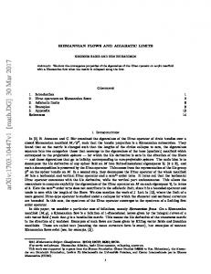
Forum on recent developments in Volume Reconstruction techniques applied to 3D fluid and solid mechanics Calibration law: It is not clear how the raw data r computed from the Kinect are related to the true distance z to the sensor. To answer this question, we acquired a set of range data for known distance-tosensor z. We plot z = f (r) in Figure 1.A. These results suggest the need to correct the raw values using a tangent law of the form z = a tan(br + c) + d. We estimated the parameters (a, b, c, d) by minimising the sum of the square errors between the actual distances z and the estimated distances a tan(br + c) + d using a gradient descent algorithm. The estimation leads to a residual error of 1.13mm2 . Projection model: We modeled the geometry of the sensor as a projection model in its simplest form which depends only on a focal length that we estimated equal to 587 pixels. Quantisation error: The raw data given by the sensor are encoded on 11-bits. We computed the mean quantisation error as the mean error R zmax between the true distance d and its nearest value given by the quantification process i.e. zmax 1−zmin z=z minr∈N |a tan(br + c) + d − z|dz which was 0.6 mm in the min range of interest (680 to 780 mm). Concerning the horizontal dimension, the magnification coefficient was about one mm per pixel near the optical axis.
Fig. 1. Experimental characterisation the sensor. A : true distance z as a function of the kinect raw data. Black dots are the measured points and the red curve is the fitted tangent calibration law. B: estimation of slopes from 3 points, red lines indicate actual slopes and black ones indicate estimated slopes. C: estimation of a sinusoidal surface, the red curves indicate the actual sinusoid and the black dots indicate the z estimated from Kinect data.
2.2 Experimental characterisation with solid surfaces
Pixel-wise error: We acquired a set of solid surfaces (from flat to quickly varying sinus-like surfaces) at different elevations and then we used the calibration law to estimate the surface-sensor distances. We obtained a mean error of about 0.9 mm with standard deviation 0.03 mm2 for each kind of surfaces. Shape recovering: We investigated the ability of the sensor to recover known geometrical patterns. In particular, we noticed that the the sensor is able to recover surfaces with steep slopes and to capture wave-like patterns of small spatial periods (< 20 mm) and small amplitudes (< 2 mm). Figure 1.B and 1.C show examples of estimated point sets. 2.3 Experimental characterisation with liquid surfaces
Since water was used as a working liquid, liquid’s light diffusivity was enhanced by the addition of white dye. We showed that errors coming from observations of solid and liquid surfaces are comparable when the attenuation coefficient of the liquid is larger than 113 m−1 . We noticed that when
Forum on recent developments in Volume Reconstruction techniques applied to 3D fluid and solid mechanics observing bright surfaces (which includes the water surfaces we studied), the sensor is unable to provide a depth data for some pixels. For an acquisition of a moving water surface in laboratory, this phenomenon affected about 1% of the pixels.
3 Applications In this section, we illustrated the usefulness of the Kinect data on two applications involving freesurface flows. 3.1 3D reconstructions
In a first step, we performed 3D reconstructions of moving liquid surfaces captured by the Kinect. Figure 2 shows a 3D temporal reconstruction of a wave. These results indicate that the Kinect was able to track waves with a good accuracy.
Fig. 2. 3D reconstruction from Kinect data. Left : picture of the experimental setting. Right : 3D reconstruction of a wave from Kinect acquisitions at t = 0.15, 0.3, 0.45 and 0.6 second. All the scales are in millimeters.
3.2 Assimilation
In a second step, we demonstrated on synthetic data the possibility to estimate both time-dependent geometry and velocity field associated to a free-surface flow from a simple temporal sequence of Kinect-like range images using a data-assimilation method and an appropriate dynamic model. More specifically, we modeled the studied system as: p =N(xinit , R0 ) x0 p xt |xt−1 ,...,x0 =p xt |xt−1 = N( f (xt−1 ), Rt ) py |x ,...,x =py |x = N(h(xt ), Qt ) t t 0 t t where: – – – –
xt is the elevation and horizontal velocity at time t in a 100×100 discretised space (hidden state), yt is the observed depth image at time t (observation), f propagates the state xt−1 at time t−1 to time t (dynamic model). Here f is a shallow-water model. h produces the observation yt from the state xt (observation model). Here h is implemented using raytracing methods. – Rt and Qt are the covariance matrices associated to the model errors and to the observation errors.
From this formulation, we estimated sequentially the posteriors p x0...t |y1...t (t ∈ [1, T ]) using a weighted ensemble Kalman filter [3] whose Kalman gain is computed from filtered empirical covariance matrices [4]. To assess the method, we generated sequences of flows from a shallow-water model and used it to generate Kinect-like observations synthetically. Then, we used the assimilation method to estimate the flows from these synthetic observations and we compared the obtained flows to the ground truth ones. Figure 3 and 4 show two results of such estimations. For both examples, the mean initial state xinit is a flat level and a null velocity and an observation is assimilated each 0.03s
Forum on recent developments in Volume Reconstruction techniques applied to 3D fluid and solid mechanics (that corresponds to 10 iterations of the dynamic model) using 100 ensemble members. In Figure 3, we considered the case where a small quantity of water fall at the center of a container at t = 0 and generates a wave. In Figure 4, we considered the case where from t = 0 to t = 0.015s, a wave of constant speed enters into a channel of nonconstant width. These results illustrate potential uses of the method and show its ability to recover both elevation and velocity from sequences of depth observations. The ratio between the energy of estimation errors (with respect to the ground truth) and the energy of the ground truth signal is about 14% for the elevation component and 18% for the velocity component. 10
10
10
20
20
20
30
30
30
40
40
40
50
50
50
60
60
60
70
70
70
80
80
80
90
90
100 10
20
30
40
50
60
70
80
90
100 100
90
10
20
30
40
50
60
70
80
90
100 100
10
20
30
40
50
60
70
80
90
100
Fig. 3. Estimation of the elevation and velocity field of a free surface flow by assimilating synthetic Kinectlike data. From left to right: i) Kinect-like observation at t = 8 × 0.03s of a wave generated by a water falling at the center of the container at t = 0, ii) estimated elevation (color map) and velocity (arrows) at t = 8 × 0.03s, iii) ground truth elevation and velocity at t = 8 × 0.03s. 10
10
10
20
20
20
30
30
30
40
40
40
50
50
50
60
60
60
70
70
70
80
80
80
90
90
100 10
20
30
40
50
60
70
80
90
100 100
90
10
20
30
40
50
60
70
80
90
100 100
10
20
30
40
50
60
70
80
90
100
Fig. 4. Estimation of the elevation and velocity field of a free surface flow by assimilating synthetic Kinectlike data. From left to right: i) Kinect-like observation at t = 19 × 0.03s of a wave evolving in a channel, ii) estimated elevation (color map) and velocity (arrows) at t = 19 × 0.03s, iii) ground truth elevation and velocity at t = 19 × 0.03s.
4 Conclusion The conclusions of this work are twofold. Firstly, the Kinect sensor is able to capture observations of wave-like surfaces with wavelengths and amplitudes sufficiently small to support applications such as flow monitoring or medium/large scale flows characterisation. Secondly, first results indicate the ability of stochastic data assimilation methods to estimate both the time dynamic surface elevation and velocity from depth images having characteristics close to the one of the Kinect. Notice that all the presented results characterise acquisitions within an area near the image center and from a short range. Future works will consist in investigating the data assimilation technique with real Kinect data and over larger ranges (the Kinect sensor is able to provide data up to 13 meters).
References 1. 2. 3. 4.
P.J. Cobelli, A. Maurel, V. Pagneux and P. Petitjeans, Exp. Fluids, 36-47, (2009) pp. 1037-1047. S.F. Bradford, B.F. Sanders, Journal of Hydraulic Engineering 128, (2002) pp. 289-298. N. Papadakis, E. M´emin, A. Cuzol, N. Gengembre. Tellus-A, (2010) P L Houtekamer, Herschel L Mitchell. Monthly Weather Review (1998)