easy, implementing a concurrent system by composing syn- chronous modular ..... mental result of Keller [7] on the deterministic operation of a system in an.
From Concurrent Multiclock Programs to Deterministic Asynchronous Implementations Dumitru Potop-Butucaru
Robert de Simone Yves Sorel INRIA, France {FirstName.LastName}@inria.fr
Abstract We propose a general method to characterize and synthesize correctness-preserving, asynchronous wrappers for synchronous processes on a globally asynchronous locally synchronous (GALS) architecture. Based on the theory of weakly endochronous systems, our technique uses a compact representation of the abstract synchronization configurations of the analyzed process to determine a minimal set of synchronization patterns generating all possible reactions.
1 Introduction Synchronous programming is nowadays a widely accepted paradigm for the design of critical applications such as digital circuits or embedded software [3], especially when a semantic reference is sought to ensure the coherence between the implementation and the various simulations. The synchronous paradigm supports a notion of deterministic concurrency which facilitates the functional modeling and analysis of embedded systems. While modeling a synchronous process or module can be easy, implementing a concurrent system by composing synchronous modular specifications is often hardened by the need of preserving global synchronizations in the model of the system. These synchronization artifacts need most of the time to be preserved, at least in part, in order to ensure functional correctness when the behavior of the whole system depends on properties such as the arrival order of events on different channels, or the presence or absence of an event at a certain instant. We address this issue and focus on the characterization and synthesis of wrappers that control the execution of synchronous processes in a GALS architecture. Our aim is to preserve the functional properties of individual synchronous processes deployed on an asynchronous execution environment. To this aim, we shall start by considering a multiclocked or polychronous model of computation and lay the
Jean-Pierre Talpin
proper theoretical background to finally establish properties pertaining on the assurance of asynchronous implementability. Our technique is mathematically founded on the theory of weakly endochronous systems, due to Potop, Caillaud, and Benveniste [11]. Weak endochrony gives a compositional sufficient condition establishing that a concurrent synchronous specification exhibits no behavior where information on the absence of an event is needed. Thus, the synchronous specification can safely be executed with identical results in any asynchronous environment (where absence cannot be sensed). Weak endochrony thus gives a latencyinsensitivity and scheduling-independence criterion. In this paper, we propose the first general method to check weak endochrony on multi-clock synchronous programs. The method is based on the construction of so-called generator sets. Generator sets contain minimal synchronization patterns that characterize all possible reactions of a multi-clocked program. These sets are used to check that a specification is indeed weakly endochronous, in which case they can be used to generate the GALS wrapper. In case the specification is not weakly endochronous, the generators can be used to generate intuitive error messages. Thus, we provide an alternative to classical compilation schemes for multi-clock programs, such as the clock hierarchization techniques used in Signal/Polychrony [1]. Outline. The paper is organized as follows: Section 2 and Section 3 give an intuition of the problem addressed in this paper together with references to previous work and an idea of the desired solution. Section 4 defines the formalism that will support our presentation. Section 5 summarizes the original theory of [11] and adapts it to our framework. Section 6 defines novel algorithms to determine if a specification is weakly endochronous. We conclude in Section 7.
2 Multiclock synchronous system We use a small, intuitive example to present our problem, the desired result, and the main implementation is-
sues. The example, pictured in Fig. 1, is a simple reconfigurable adder, where two independent single-word ALUs can be used either independently, or synchronized to form a double-word ALU. The choice between synchronized and non-synchronized mode is done using the SYNC signal. The carry between the two adders is propagated through the Boolean C wire whenever SYNC is present. I1
to model cases where only parts of the process compute. We will say that a signal is present in a reaction when it has a value in DS . Otherwise, we say that it is absent. Absence is simply represented with value ⊥, which is appended to all domains DS⊥ = DS ∪ {⊥}. Formally, a reaction of the process is a valuation of its signals into their extended domains DS⊥ . We denote with R the set of all such valuations. The support of a reaction r, denoted supp(r), is the set of present signals. For instance, the support of reaction 4 in Fig. 2 is {I1, I2, O1, O2}. In a reaction r, we distinguish the input event, which is the restriction r |I(EXAMPLE) of r to input signals, and the output event, which is the restriction r |O(EXAMPLE) to output signals. In many cases we are only interested in the presence or absence of a signal, because it transmits no data, just synchronization (or because we are only interested in synchronization aspects). To represent such signals, the Signal language [6] uses a dedicated event type of domain Devent = {•}. We follow the same convention: In our example, SYNC has type event. To represent reactions, we use a set-like convention and omit signals with value ⊥. In Fig. 2, the signal types are SY N C : event, O1, O2 : integer, I1, I2 : integer pair, C : Boolean. Reaction 4 is denoted (I1(9,9) , O18 , I2(0,0) , O20 ). The stuttering reaction assigning ⊥ to all signals is denoted ⊥. Reaction 5 is a stuttering reaction.
O1 ADD1
C
SYNC
ADD2 I2
O2
Figure 1. Data-flow of a configurable adder.
1
We consider a discrete model of time, where executions are sequences of reactions, indexed by a global clock. Given a synchronous specification (also called process), a reaction is a valuation of the input, output and internal (local) signals of the process. Fig. 2 gives a possible execution of our example. We shall denote with V(P ) the finite set of signals of a process P . We shall distinguish inside V(P ) the disjoint sub-sets of input and output signals, respectively denoted I(P ) and O(P ). Clock
1
2
3
4
5
6
7
I1 O1 SYNC C I2 O2
(1,2) 3 ⊥ ⊥ ⊥ ⊥
⊥ ⊥ ⊥ ⊥ ⊥ ⊥
(9,9) 8 • 1 (0,0) 1
(9,9) 8 ⊥ ⊥ (0,0) 0
⊥ ⊥ ⊥ ⊥ ⊥ ⊥
(2,5) 7 • 0 (1,4) 5
⊥ ⊥ ⊥ ⊥ (2,3) 5
3 Deterministic asynchronous implementation We consider a synchronous process, and we want to execute it in an asynchronous environment where inputs arrive and outputs depart via asynchronous FIFO channels with uncontrolled (but finite) communication latencies. To simplify, we assume that we have exactly one channel for each input and output signal of the process. We also assume a very simple correspondence between messages on channels and signal values: Each message on a channel corresponds to exactly one value (not absence) of a signal in a reaction. In particular, no message represents absence. We assume that the execution of the synchronous process is a cyclic repetition of 3 steps: 1. assembling asynchronous input messages arriving onto the input channels into a synchronous input event acceptable by the process, 2. triggering a reaction of the process for the reconstructed input event, and 3. transforming the output event of the reaction into messages onto the output asynchronous channels.
Figure 2. A synchronous run of the adder If we denote with EXAMPLE our configurable adder, then V(EXAMPLE) = I(EXAMPLE) = O(EXAMPLE) =
{I1, I2, SY N C, O1, O2, C} {I1, I2, SY N C} {O1, O2}
All signals are typed. We denote with DS the domain of a signal S. Not all signals need to have a value in a reaction,
In order to achieve deterministic execution,2 the main difficulty lies in step (1), as it involves the potential recon-
1 To
simplify figures and notations, we group both integer inputs of ADD1 under I1, and both integer inputs of ADD2 under I2. This poses no problem because from the synchronization perspective of this paper the two integer inputs of an adder have the same properties.
2 Like in [10], determinism can be relaxed here to predictability – the fact that the environment is always informed of the choices made inside the process. While this involves no changes in the following technical results, we preferred a simpler presentation.
2
struction of signal absence, whereas absence is meaningless in the chosen asynchronous framework. Reconstructing reactions from asynchronous messages must be done in a deterministic fashion, regardless of the message arrival order. This is not always possible. Assume, like in Fig. 3, that we consider the inputs of Fig. 2 without synchronization information. I1 O1 SYNC C I2 O2
for checking weak endochrony of real-life (real-size) specifications.
3.1 Previous work. Motivation The most developed notions identifying classes of implementable processes are the concepts of latency-insensitive systems of Carloni et al. [4] and the endochronous systems of Benveniste et al. [2, 6]. The latency-insensitive systems are those featuring no signal absence. Transforming processes featuring absence, such as our example of Figures 1 and 2, into latency-insensitive ones amounts to transforming the presence/absence of a signal into a true/false value that is sent and received as an asynchronous message. This is easy to check and implement, but often results in an unneeded communication overhead due to the absence messages. The endochronous systems and the related hardwarecentric generalized latency-insensitive systems [14] are those where the presence and absence of all signals can be incrementally inferred starting from the state and from signals that are always present. For instance, Fig. 4 presents a run of an endochronous system obtained by transforming the SYNC signal of our example into one that carries values from 0 to 3: 0 for ADD1 executing alone, 1 for ADD2 executing alone, 2 for both adders executing without communicating (C absent), and 3 for the synchronized execution of the two adders (C present). Note that the value of SYNC determines the presence/absence of all signals.
(1,2) (9,9) (9,9) (2,5) 3 8 8 7 •• 10 (0,0) (0,0) (1,4) (2,3) 1 0 5 5
Figure 3. Corresponding asynchronous run. No synchronization exists between the various signals, so that correctly reconstructing synchronous inputs from the asynchronous ones is impossible
The adder ADD1 will then receive the first value (1, 2) on the input channel I1 and • on SYNC. Depending on the arrival order, which cannot be determined, any of the reactions (I1(1,2) , O13 , SY N C • , C 0 ) or (I1(1,2) , O13 ) can be executed, leading to divergent computations. The problem is that these two reactions are not independent, but no value of a given channel allows to differentiate one from the other (so one can’t deterministically choose between them in an asynchronous environment). We have seen in the previous section that deterministic input event reconstruction is impossible for some synchronous processes. This means that a methodology to implement synchronous processes on an asynchronous architecture must rely on the (implicit or explicit) identification of some class of processes for which reconstruction is possible. Then, giving a deterministic asynchronous implementation to a random synchronous process can be done in two steps:
Clock
1
2
3
4
5
I1 O1 SYNC C I2 O2
(1,2) 3 0 ⊥ ⊥ ⊥
(9,9) 8 3 1 (0,0) 1
(9,9) 8 2 ⊥ (0,0) 0
(2,5) 7 3 0 (1,4) 5
⊥ ⊥ 1 ⊥ (2,3) 5
Figure 4. Endochronous solution Checking endochrony consists in ordering the signals of the process in a tree representing the incremental presence inference process (the signals that are always read are all placed in the tree root). The compilation of the Signal/Polychrony language is currently founded on a version of endochrony [1]. The endochronous reaction reconstruction process is fully deterministic, and the presence of all signals is synchronized w.r.t. some base signal(s) in a hierarchic fashion. This means that no concurrency remains between subprocesses of an endochronous process. For instance, in the endochronous model of our adder, the behavior of the two adders is synchronized at all instants by the SYNC signal
1. transforming the initial process, through added synchronizations and/or signals, so that it belongs to the implementable class, and then 2. generating an implementation for the transformed process. The choice of the class of implementable processes is therefore essential. On one hand, choosing a small class can highly simplify analysis and code generation in step (2). On the other, small classes of processes result in heavier synchronization added to the process in step (1). Our choice, justified in the next section, is the class of weakly endochronous processes. This paper proposes a technique 3
putations,3 while adding the supplementary synchronization needed to ensure deterministic execution in an asynchronous environment. Weak endochrony is preserved by synchronous composition, thus supporting incremental development. However, the lack of a practical technique for checking and/or synthesizing weak endochrony limited its use in practice until now. We use the high-level multi-clock synchronous data-flow language Signal [1] to demonstrate the applicability of our technique. This language allows a simple representation of clock synchronization constraints we are interested in. Like other synchronous data-flow formalisms, such as Lustre, Scade, Lucid, that could also have been considered, Signal gives an implicit representation of states that is most convenient (yet not mandatory) for a direct illustration of our technique.
(whereas in the initial model the adders can function independently whenever SYNC is absent). By consequence, using endochrony as the basis for the development of systems with internal concurrency has 2 drawbacks: • Endochrony is non-compositional (synchronization code must be added even when composing processes sharing no signal). • Specifications and implementations/simulations are over-synchronized. Weak endochrony, due to Potop, Caillaud, and Benveniste [11] and presented in Section 5, generalizes endochrony by allowing both synchronized and nonsynchronized (independent) computations to be realized by a given process. Fig. 5 presents a run of a weakly endochronous system obtained by replacing the SYNC signal of our example with two input signals:
4.1 Finite stateless abstraction We define our decision procedure for weak endochrony on the finite-data stateless abstraction of Signal programs that is already used in existing compilers. This subset is defined by (1) a restriction to finite data types and (2) the abstraction of delay equations (sole to introduce implicit state transition) by synchronization constraints (between the signals of a delay equation). For programs featuring infinite data and delays (e.g., integer, float) the construction of an finite-data stateless abstraction is done by a procedure of the Signal compiler that is detailed in [9]. Given that a Signal specification needs not be functionally complete, the abstraction can be represented as a Signal process (and it is derived through simple transformations of the Signal source). The stateless abstraction does not mean all state information is lost. The abstraction procedure automatically conserves some of the underlying synchronization information, and the programmer can force the preservation of as much information as needed through the addition of socalled clock constraints (defined in Section 4.3.1), which are preserved by the abstraction procedure. For instance, activation conditions such as the ones used in the compilation of Esterel [13] can be easily preserved in this way. However, the abstraction means that: (1) Certain weakly endochronous processes are rejected, as the analysis cannot determine it and (2) The code generated for a weakly endochronous process may be over-synchronized.
• SYNC1, of Boolean type, is received at each execution of ADD1. It has value 0 to notify that no synchronization is necessary, and value 1 to notify that synchronization is necessary and the carry signal C must be produced. • SYNC2, of Boolean type, is received at each execution of ADD2. It has value 0 to notify that no synchronization is necessary, and value 1 to notify that synchronization is necessary and the carry signal C must be read. The two adders are synchronized when SYNC1=1 and SYNC2=1, corresponding to the cases where SYNC=• in the original design. However, the adders function independently elsewhere (between synchronization points). I1 O1 SYNC1
(1,2) 3 0
(9,9) 8 1
C SYNC
1 •
SYNC2 I2 O2
1 (0,0) 1
(9,9) 8 0
(2,5) 7 1 0 • 0 (0,0) 0
1 (1,4) 5
0 (2,3) 5
Figure 5. Weakly endochronous solution
4.2 Process structure In Signal, a specification is a process, whose definition may involve other processes, hierarchically. Fig. 6 gives the Signal process corresponding to the configurable adder of
4 Multiclock Specification in Signal The use of weakly endochronous processes allows the preservation of the independence of non-synchronized com-
3 So
4
that later analysis or implementation steps can exploit it.
4.3.1 Clocks. Clock Constraints
Fig. 1. A process is formed of a header defining its name, an interface specification, a data-flow specification, and a local declaration section. In our example, the top-level process is named EXAMPLE. Its interface defines 3 input signals (SYNC, I1, and I2), identified with “?”, and 2 output signals (O1 and O2), identified with “!”. Our example has no state, and the infinite type signals (I1, I2, O1, O2) have been replaced with signals of type event by the abstraction procedure. The Boolean type of the carry C has also been transformed into event, because it is computed from I1 (we need to preserve determinism). 1 2 3 4 5 6 7 8 9 10 11 12 13 14
The clock of a signal S is another signal, denoted ∧ S, of type event, which is present whenever S is present. Clock signals are used to specify clock constraints. The most common clock constraints are identity, inclusion, and exclusion. Lines 8 and 9 of Fig. 6, which gives the constraints of ADD1, illustrates clock equality and inclusion. The equation “I1∧ =O1” specifies that signal I1 is present in a reaction iff O1 is present. In other terms, whenever inputs arrive, the adder produces an output. The next equation requires that I1 is present in reactions where SYNC is present. Otherwise said, ∧ SYNC is included in ∧ I1. The last equation states that the carry value C is emitted by ADD1 whenever SYNC is present. The definition of ADD2 is similar. The difference is that the carry signal C is here an input, and not an output like in ADD1. Clock exclusion is not used in our example. Writing “S1∧ #S2” requires that S1 and S2 are never present in the same reaction.
process EXAMPLE = (? event SYNC,I1, I2 ! event O1, O2 ) (| (O1,C) := ADD1 (SYNC,I1) | O2 := ADD2 (SYNC,I2,C) |) where event C ; process ADD1 = (? event SYNC, I1 ! event O1, C ) (| I1 ˆ= O1 | SYNC ˆ< I1 | C ˆ= SYNC |) ; process ADD2 = (? event SYNC, I2, C ! event O2 ) (| I2 ˆ= O2 | SYNC ˆ< I2 | C ˆ= SYNC |) ; end ;
4.3.2 Stateless Signal primitive language The following statements are the primitives of the Signal language sub-set we consider. The delay primitive of the full language, “X:=Y$ init V” 4 , is simply abstracted by its synchronization requirement “X∧ =Y”. The assignment equation “X:=f(Y1,...,Yn)” states that all the signals have the same clock, and that the specified equality relation holds at each instant where the signals are present. Equation “X:=Y” is a particular case of assignment. It specifies the identity of X and Y. Signal Y can also be replaced with a data-flow expression built using the following operators: The operator when performs conditional downsampling. The signal “X when C” is equal to X whenever the boolean signal C is present with value true. Otherwise, it is ⊥. The shortcut for “∧ C when C” is “when C”. For instance, in Fig. 7, “when SYNC1=1” is a signal of type event that is present when signal SYNC1 is present with value 1. The operator default merges two signals of the same type, giving priority to the first. The signal “X default Y” is present whenever one of X or Y is present. It is equal to X whenever X is present, and is equal to Y otherwise.
Figure 6. The Signal process of the configurable adder in Fig. 1
The data-flow specification of EXAMPLE consists of two equations, which define the interconnections between ADD1, ADD2, and the environment. The local definition section defines the internal signal C, and the processes ADD1 and ADD2. The hierarchy of processes allows the structuring of a specification and the definition of signal scopes that mask internal signals. Process EXAMPLE using process ADD1 in its data-flow intuitively corresponds to replacing each instance of ADD1 in EXAMPLE with its data-flow with the internal signals of ADD1 being masked.
4.3 Data-flow
5 Weak endochrony
The data-flow specification of a process is formed of equations defining constraints between the signals of the process. Any reaction satisfying all the equations of a process P is a valid reaction of P . We denote with R(P ) the set of all the reactions of P . The use of a constraint language allows us to easily manipulate functionally incomplete specifications.
The theory of weakly endochronous (WE) systems [11], gives criteria establishing that a synchronous presentation hides a behavior that is fundamentally asynchronous and 4 X is defined by V the first time Y occurs and then takes the previous value of Y
5
deterministic. Absence information is not needed, which guarantees the deterministic implementability of the synchronous specification in an asynchronous environment.5 Absence not being needed in computations means that reactions sharing no common present value can be executed independently (without any synchronization). Absence is treated as a don’t care value imposing no synchronization constraint (as opposed to present values).
Definition 1 (stateless weak endochrony) We say that process P is weakly endochronous its set of reactions R(P ) is closed under the operations associated to the previously-defined domain structure: intersection, union, and difference of non-contradictory reactions. Atoms. From our point of view oriented towards automated analysis, it is most interesting that any behavior of a WE system can be decomposed into atomic transitions, or atoms. Formally, the set of atomic reactions of P , denoted Atoms(P ) is the set of the smallest (in the sense of ≤) reactions of R(P ) different from ⊥. The set of atomic transitions is characterized by two fundamental properties: non-interference and generation.
process EXAMPLE2 = (? boolean S1, S2; event I1,I2 ! event O1,O2 ) (| (O1,O2) := EXAMPLE (when S1, I1, I2) | when S1 ˆ= when S2 |) where process EXAMPLE = the process in Fig. 6 end
Theorem 1 (atom set characterization) A stateless process P is weakly endochronous if and only if there exists a set of reactions A ⊆ R(P ) such that:
Figure 7. A weakly endochronous refinement of process EXAMPLE is obtained by limiting the use of signal absence (when compared to the other solutions)
Generation: The union of non-interfering atoms W generates all the reactions of R(P ): R(P ) = { K | K ⊆ G∧ ⊲⊳ K}. Non interference: Two distinct atoms a1 , a2 ∈ A, a1 6= a2 are either contradictory or independent.
This property suggests a natural organization of the possible values of a signal S as a Scott domain defined by ⊥ ≤ v, for all v ∈ DS . The domain structure on particular signals induces a product partial order ≤ on reactions with r1 ≤ r2 if and only if supp(r1 ) ⊆ supp(r2 ) and r1 (v) = r2 (v) for all v ∈ supp(r1 ). We say of two reactions r1 and r2 that they are noncontradictory, written r1 ⊲⊳ r2 , if r1 (v) = r2 (v) for all v ∈ supp(r1 ) ∩ supp(r2 ). Otherwise, we say that the reactions are contradictory, written r1 6⊲⊳ r2 . Given a set of reactions K, we shall say that it is non-contradictory, denoted ⊲⊳ K if any two reactions of K are non-contradictory. The least upper bound and greatest lower bound induced by the order relation are respectively denoted with ∨ and ∧, and called union and intersection of reactions. If r1 ⊲⊳ r2 , both r1 ∨ r2 and r1 ∧ r2 are defined, and we can also define the difference r1 \r2 , which has support supp(r1 )\supp(r2 ) and equals W r1 on its support. For a set K with ⊲⊳ we denote ∨K = r∈K r. Weak endochrony is defined in an automata-theoretic framework. We simplify it here according to our stateless abstraction:
Axiom (Non interference) implies that as soon as two atoms are not independent, they can be distinguished by a present value (not absence), meaning that choice between them can be done in an asynchronous environment. The characterization of Theorem 1 corresponds to the case where no distinction is made between input, output and internal signals of a system (which is the case in [11]). As we seek to obtain deterministic asynchronous implementations for Signal programs, we require that the choice between any two contradictory atoms can be done based on input signal values.6 Formally: Input choice: For any two contradictory atoms a1 , a2 ∈ A, there exists s ∈ V(P ) such that ai (s) 6= ⊥, i = 1, 2, and a1 (s) 6= a2 (s).
6 Checking weak endochrony According to Theorem 1, checking weak endochrony is determining when an atom set can be constructed for a given process. We follow this approach by determining for each process P one minimal set of supplementary synchronizations (under the form of signal absence constraints) allowing the construction of a generator set with atom-like properties. Process P is weakly endochronous iff the generators are free of forced absence constraints.
5 The intuition behind weak endochrony is that we are looking for systems where (1) all causality is implied by the sequencing of messages on communication channels, and (2) all choices are visible as choices over the value (and not present/absent status) of some message. As explained in [10], the axioms of weak endochrony can be traced down to the fundamental result of Keller [7] on the deterministic operation of a system in an asynchronous environment. Moreover, WE systems are synchronous Kahn processes, and weak endochrony extends to a synchronous framework the classical trace theory [8].
6 To achieve predictability, choice can be done on input or output signal values.
6
6.1 Signal absence constraints
Definition 3 (Fully constrained generator set) A generator set G of process P is called fully constrained if each atom represents all absence constraints associated to it. V Formally, for all g ∈ G we have: g = {r | r ∈ R(P ) ∧ g ≤ r}.
For processes P that are not weakly endochronous, the set of reactions R(P ) is not closed under the operations ∨, ∧, \ defined in the previous section, meaning that we cannot use generation properties to represent R(P ) in a compact fashion. This is due to the fact that the model does not allow the representation of absence constraints, which are needed in order to represent the reaction to signal absence. To allow compact representation, we enrich the model with absence constraints under the form of constrained absence ⊥ ⊥ signal values which are added to the domain of each signal. An extended reaction r sets signal S to ⊥ ⊥ to represent the fact that upon union (∨) the signal S must remain absent. This new value represents the classical synchronizing absence of the synchronous model, which must be preserved at composition time. However, we are not interested in fully reverting to a synchronous setting, but in preserving as few synchronizations as needed to allow deterministic asynchronous execution. We denote with DS⊥⊥ = DS⊥ ∪ {⊥ ⊥} the new domain with ⊥ ≤ ⊥ ⊥. The operators ∧, ∨, and \ are extended accordingly. We denote with R⊥⊥ the set of valuations of the signals over the extended domains. On R⊥⊥ we can extend the operators ∧, ∨, \, and ⊲⊳. We define the operator [] : R⊥⊥ → R that removes absence constraints (replaces ⊥ ⊥ values with ⊥). We also define the converse transformation : R → R⊥⊥ that transforms all the ⊥ values of a reaction into ⊥ ⊥ values. We denote ⊥ ⊥ = ⊥ the reaction assigning ⊥ ⊥ to all signals.
Finally, we are looking for generator sets with atom-like exclusiveness properties. Definition 4 (Non-interfering generator set) A generator set G of process P is called non-interfering if for all r1 , r2 ∈ G with r1 ⊲⊳ r2 and [r1 ] ∧ [r2 ] 6= ⊥ we have r1 = r2 . Every Signal process has a fully constrained noninterfering generator set, obtained by replacing ⊥ with ⊥ ⊥ in all the reactions of R(P ). But using this representation amounts to reverting to the synchronous model, and not exploiting the concurrency of the process. We are therefore looking for least synchronized generator sets exhibiting minimal absence constraints. Definition 5 (Less synchronized generator set) Let P be a process and G1 , G2 two generator sets for P . We say that G1 is less synchronized than G2 , denoted W G1 � G2 , if for all g ∈ G there exists K ⊆ G with 2 2 1 g∈K g ≤ g2 and W [ g∈K g] = [g2 ]. The procedures of the next section will build for each process a fully constrained, non-interfering generator set that is minimal in the sense of �. Theorem 2 Let P be a process and G be a fully constrained, non-interfering generator set that is minimal in the sense of �. Then, G is weakly endochronous if and only if the set AG = {[g] | g ∈ G} satisfies the generation and non-interference properties of Theorem 1.
6.2 Generators We define in this section the notion of minimal fully constrained non-interfering set of generators of a process P , which is very similar to an atom set, except (1) it can be computed for any process P and (2) it involves absence constraints. Such generator sets will represent for us compact representations of R(P ), and the basic objects in our weak endochrony check technique. The reactions of such a generator set can be seen as tiles that can be united (when disjoint) to generate all other reactions. Generators can also be compared with the prime implicants of a logic formula – they are reactions of smallest support that generate all other reactions.
Proof sketch: If AG satisfies the given property, then according to Theorem 1 we know that P is weakly endochronous. In the other sense, assume A is the set of atoms of the weakly endochronous process P . For all a ∈ A we define ^ ga = {r | r ∈ R(P ) ∧ a ≤ r} Then, GA = {ga | a ∈ A} is a fully constrained noninterfering generator set that can be proved minimal in the sense of � (ant it is unique with this property). � If a process is not weakly endochronous, then there may exist several minimal non-interfering generator sets. We provide here a technique allowing the construction of one such generator set. Our technique works inductively: We compute a minimal generator set for each statement in a bottom-up fashion following the syntax of the process. We
Definition 2 (Generator set) Let P be a process. A set G ⊆ R⊥⊥ of partial reactions such that [g] 6= W⊥ for all g ∈ G is a generator set of R(P ) if R(P ) = {[ g∈K g] | K ⊆ G∧ ⊲⊳ K}. As we are building our generator sets incrementally, it is essential they preserve all the synchronization information of the process, including all absence constraints. Such generator sets are called fully constrained. 7
GV X:=Y default Z =
are of only two types: parallel composition and sumodule instantiation. This section deals with parallel composition: The main algorithm is ParallelComposition, which computes a minimal generator set of p | q starting from minimal generator sets of p and q. The signal scoping realized by subprocess instantiation must be ignored, meaning that the local signals of the generators of the sub-process are treated as local signals of the instantiating process itself. This is necessary if the goal is multi-task code generation, because hiding local signals can hide actual dependencies and render non-interfering reactions that are interfering in the sub-process. For space reasons, we relegate to Appendix A the routine allowing the hiding of local signals at the level of subprocess instantiation (which may be useful for verification purposes).
= {(X v , Y v , Z w ) | v ∈ DX , w ∈ DX ∪ {⊥ ⊥}} ∪ {(X v , Y ⊥⊥ , Z v ) | v ∈ DX } ∪ {(W v ) | v ∈ DX , W ∈ V \ {X, Y, Z}} GV X:=Y when Z = =
{(X v , Y v , Z 1 ) | v ∈ DX } ∪ {(X ⊥⊥ , Y v , Z 0 ) | v ∈ DX ∪ {⊥ ⊥}} ∪ {(X ⊥⊥ , Y v , Z ⊥⊥ ) | v ∈ DX } ∪ {(W v ) | v ∈ DX , W ∈ V \ {X, Y, Z}}
GV X:=f(Y
1 ,...,Yn )
=
= {(X f (v1 ,...,vn ) , Y1 v1 , . . . , Yn vn ) | ∀i : vi ∈ DYi } ∪ {(W v ) | v ∈ DX , W ∈ V \ {X, Yi | 1 ≤ i ≤ n}}
Function 1 ParallelComposition Input: Gp , Gq : generator set Output: Gp|q : generator set G′ ← ∅ for all g ∈ Gp do ParallelCompositionAux(g,⊥,Gp ,Gq ,G′ ) Gp|q ← MinimizeSynchronization(G′ )
Figure 8. Minimal generator sets for primitive Signal equations
GV X∧ =Y
=
{(X v , Y w ) | v ∈ DX , w ∈ DY } ∪ {(W v ) | v ∈ DW , W ∈ V \ {X, Y }}
GV X∧